Topics 6-9

Question 1

Describe financial correlation risk and the areas in which it appears in finance

Answer 1

Correlation risk measures the risk of financial loss resulting from adverse changes in correlations between financial or nonfinancial assets.

An example of financial correlation risk is the negative correlation between interest rates and commodity prices. If interest rates rise, losses occur in commodity investments.

• Another example* of this risk occurred during the 2012 Greek crisis. The positive correlation between Mexican bonds and Greek bonds caused losses for investors of Mexican bonds.
• Nonfinancial assets* can also be impacted by correlation risk.

Financial correlations can be categorized as static or dynamic.

Static financial correlations do not change and measure the relationship between assets for a specific time period.

Examples of static correlation measures are value at risk (VaR), correlation copulas for collateralized debt obligations (CDOs), and the binomial default correlation model.

Dynamic financial correlations measure the comovement of assets over time.

Examples of dynamic financial correlations are pairs trading, deterministic correlation approaches, and stochastic correlation processes.

There are many areas in finance that have financial correlations. Five common finance areas where correlations play an important role are:

1. investments,
2. trading,
3. risk management,
4. global markets, and
5. regulation.

Question 2

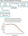
Correlation risk in structured products

Answer 2

Structured products are becoming an increasing area of concern regarding correlation risk.

If Deutsche Bank and France default (worst case scenario), the investor loses the entire $ 1 million investment.

If there is positive correlation risk between Deutsche Bank and France, the investor has wrong-way risk (WWR). The higher the correlation risk, the lower the CDS spread, s. The increasing correlation risk increases the probability that both the French bond (reference asset) and Deutsche Bank (counterparty) default.

The dependencies between the CDS spread, s, and correlation risk may be nonmonotonous. This means that the CDS spread may sometimes increase and sometimes decrease if correlation risk increases.

Question 3

Covarience and correlation coefficient

Answer 3

Question 4

Relationship of Return/Risk Ratio and Correlation

Answer 4

Question 5

Correlation in Trading with Multi-Asset Options

Answer 5

Correlation trading strategies involve trading assets that have prices determined by the comovement of one or more assets over time. Correlation options have prices that are very sensitive to the correlation between two assets and are often referred to as multi-asset options.

Question 6

Quanto Option

Answer 6

The quanto option is another investment strategy using correlation options. It protects a domestic investor from foreign currency risk. However, the financial institution selling the quanto call does not know how deep in the money the call will be or what the exchange rate will be when the option is exercised to convert foreign currency to domestic currency. Lower correlations between currencies result in higher prices for quanto options.

Question 7

Describe the structure, uses, and payoffs of a correlation swap

Answer 7

A correlation swap is used to trade a fixed correlation between two or more assets with the correlation that actually occurs. The correlation that will actually occur is unknown and is referred to as the realized or stochastic correlation. Figure 6 illustrates how a correlation swap is structured. In this example, the party buying a correlation swap pays a fixed correlation rate of 30%, and the entity selling a correlation receives the fixed correlation of 30%.

Another example of buying correlation is to buy call options on a stock index (such as the Standard & Poor’s 500 Index) and sell call options on individual stocks held within the index. If correlation increases between stocks within the index, this causes the implied volatility of call options to increase. The increase in price for the index call options is expected to be greater than the increase in price for individual stocks that have a short call position.

An investor can also buy correlation by paying fixed in a variance swap on an index and receiving fixed on individual securities within the index. An increase in correlation for securities within the index causes the variance to increase. An increase in variance causes the present value of the position to increase for the fixed variance swap payer (i.e., variance swap buyer).

Currently there is no industry-standard valuation model for correlation swaps.

Question 8

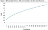
Estimate the impact of different correlations between assets in the trading book on the VaR capital charge

Answer 8

The formula for calculating VaR using the variance-covariance method (a.k.a. delta-normal method) is shown as follows.

The Basel Committee on Banking Supervision (BCBS) requires banks to hold capital based on the VaR for their portfolios. The BCBS requires banks to hold capital for assets in the trading book of at least three times greater than 10-day VaR. The trading book includes assets that are marked-to-market, such as stocks, futures, options, and swaps.

Question 9

Relationship Between VaR and Correlation for Two-Asset Portfolio

Answer 9

Question 10

Explain how correlation contributed to the global financial crisis of 2007 to 2009

Answer 10

The correlations of assets within and across different sectors and geographical regions are a major contributing factor for the financial crisis of 2007 to 2009. The economic environment, risk attitude, new derivative products, and new copula correlation models all contributed to the crisis.

Bonds within specific credit quality levels typically are more highly correlated.

While there were multiple causes of the crisis, here are the main ones:

1. Increased speculation fueled by loose credit
2. Complex credit products
3. Model risk: the new copula correlation model, which was trusted by many investors and which could presumably correlate the n(n−1)/2 assets in a structured product. Most CDOs contained 125 assets. There are 125(125−1)/2=7,750 asset correlation pairs to be quantified and managed.
4. Moral hazards: rating agencies were paid by the same companies whose assets they rated. As a consequence, many structured products received AAA ratings and gave the illusion of little price and default risk. Risk managers and regulators who lowered their standards in light of the greed and profit frenzy.
5. Increased risk appetite: around 2003, two years after the Internet bubble burst, the risk appetite of the financial markets increased, and investment banks, hedge funds, and private investors began to speculate and invest in the stock markets, commodity markets, and the real estate market.

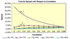
Hedge funds had shorted the equity tranche (0% to 3%) to collect the high equity tranche spread. They had then presumably hedged the risk by going long the mezzanine tranche (3% to 7%). As we can see from the figure, this hedge is flawed.

When the correlations of the assets in the CDO decreased, the hedge funds lost on both positions.

1. The equity tranche spread increased sharply; see arrow 1. Hence the fixed spread that the hedge funds received in the original transaction was now significantly lower than the current market spread, resulting in a paper loss.
2. The hedge funds lost on their long mezzanine tranche positions, since a lower correlation lowers the mezzanine tranche spread; see arrow 2. The spread that the hedge funds paid in the original transactions was now higher than the market spread, resulting in another paper loss.

Question 11

Explain the role of correlation risk in market risk and credit risk, relate correlation risk to systemic and concentration risk (explain Migration risk, Default correlation, Systemic risk, Concentration riks)

Answer 11

• Migration risk is the risk that the quality of a debtor decreases following the lowering of quality ratings.
• Default correlation is of critical importance to financial institutions in quantifying the degree that defaults occur at the same time. A lower default correlation is associated with greater diversification of credit risk. Empirical studies have examined historical default correlations across and within industries. Most default correlations across industries are positive with the exception of the energy sector. The energy sector has little or no correlation with other sectors and is, therefore, more resistant to recessions.
• Historical data suggests that default correlations are higher within industries. Creditors benefit by diversifying exposure across industries to lower the default correlations of debtors.
• Systemic risk refers to the potential risk of a collapse of the entire financial system.
• The consumer staples and pharmaceutical sector are often recession resistant as individuals continue to need basic necessities such as food, household supplies, and medications. The educational sector is also resilient as more unemployed workers go back to school for education and career changes.
• When diversification was needed most during the financial crisis, almost all stocks become more highly correlated and, therefore, less diversified. The severity of correlation risk is even greater during a systemic crisis when one considers the higher correlations of U.S. equities with bonds and international equities.
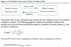
• Concentration risk is the financial loss that arises from the exposure to multiple counterparties for a specific group. Concentration risk is measured by the concentration ratio.

A lower (higher) concentration ratio reflects that the creditor has more (less) diversified default risk. For example, the concentration ratio for a creditor with 100 loans of equal size to different entities is 0.01 (= 1/100). If a creditor has one loan to one entity, the concentration ratio for the creditor is 1.0 (=1/1).

Question 12

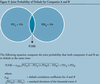
Joint Probability of Default for Companies (A and B)

Answer 12

As the concentration ratio decreases, the probability of the
worst case scenario also decreases. Both a lower concentration ratio and lower correlation coefficient reduce the joint probability of default.

Question 13

Term structure of defaults

Answer 13

• For most investment grade bonds, the term structure of default probabilities increases in time. This is because the longer the time horizon, the higher the probability of adverse internal events such as mismanagement, or adverse external events such as increased competition or a recession.
• For bonds in distress, the default term structure is typically inverse. This is because for a distressed company the immediate future is critical. If the company survives the coming problematic years, the probability of default decreases.

Question 14

Describe how equity correlations and correlation volatilities behave throughout various economic states

Answer 14

• Correlations were highest during recessions when common stocks in equity markets tend to go down together. The low correlation levels during an expansionary period suggest common stock valuations are determined more on industry and company-specific information rather than macroeconomic factors.
• Investors expect stocks to go down during a recession and up during an expansionary period, but they are less certain of direction during normal times, which results in higher correlation volatility.
• Risk managers should be cognizant of high correlation and correlation volatility levels during recessions and times of extreme economic distress when calibrating risk management models.

Question 15

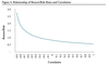
Calculate a mean reversion rate using standard regression

Answer 15

Mean reversion implies that over time, variables or returns regress back to the mean or average return. Empirical studies reveal evidence that bond values, interest rates, credit spreads, stock returns, volatility, and other variables are mean reverting.

• The stronger or faster mean reversion is expected with a higher mean reversion rate.
• From the 1972 to 2012 study, the data resulted in the following regression equation: Y = 0.27 - 0.78X

The beta coefficient of -0.78 implies a mean reversion rate of 78%. This is a relatively high mean reversion rate. Thus, if there is a large decrease (increase) from the mean correlation for one month, the following month is expected to have a large increase (decrease) in correlation.

Question 16

Calculate the autocorrelation

Answer 16

Autocorrelation measures the degree that a current variable value is correlated to past values. Autocorrelation is often calculated using an autoregressive conditional heteroskedasticity (ARCH) model or a generalized autoregressive conditional heteroskedasticity (GARCH) model. An alternative approach to measuring autocorrelation is running a regression equation. In fact, autocorrelation has the exact opposite properties of mean reversion.

Mean reversion measures the tendency to pull away from the current value back to the long-run mean. Autocorrelation instead measures the persistence to pull toward more recent historical values. The mean reversion rate for Dow stocks is 78%. Thus, the autocorrelation for a one-period lag is 22% for the same sample. The sum of the mean reversion rate and the one-period autocorrelation rate will always equal one (i.e., 78% + 22% = 100%).

Question 17

Identify the best-fit distribution for equity, bond, and default correlations

Answer 17

• The Johnson SB distribution (which has two shape parameters, one location parameter, and one scale parameter) provided the best fit for equity correlations. The Johnson SB distribution best fit was also robust with respect to testing different economic states for the time period in question. The normal, lognormal, and beta distributions provided a poor fit for equity correlations.
• The percentage change in correlation volatility prior to a recession was negative in every case except for the 1990 to 1991 recession. This is consistent with the findings discussed earlier where correlation volatility is low during expansionary periods that often occur prior to a recession.

Question 18

Evaluate the limitations of financial modeling with respect to the model itself

Answer 18

• Almost all financial models require market valuations as inputs. Unfortunately, these values are often determined by investors who do not always behave rationally. Therefore, asset values are sometimes random and may exhibit unexpected changes.
• Financial models also require assumptions regarding the underlying distribution of the asset returns. Value at risk (VaR) models are used to estimate market risk, and these models often assume that asset returns follow a normal distribution. However, empirical studies actually find higher kurtosis in return distributions, which suggest a distribution with fatter tails than the normal distribution.
• Another example of a shortcoming of financial models is illustrated with the Black-Scholes-Merton (BSM) option pricing model. The BSM option pricing model assumes strike prices have constant volatility. However, numerous empirical studies find higher volatility for out-of-the money options and a volatility skew in equity markets. Thus, option traders and risk managers often use a volatility smile with higher volatilities for out-of-the money call and put options.
• Financial models at times may fail to accurately measure risk due to mathematical inconsistencies. For example, regarding barrier options, when applying the BSM option pricing model to up-and-out calls and puts and down-and-out calls and puts, there are rare cases where the inputs make the model insensitive to changes in implied volatility and option maturity. This can occur when the knock-out strike price is equal to the strike price, and the interest rate equals the underlying asset return. Risk managers and traders need to be aware of the possibility of mathematical inconsistencies causing model risk that leads to incorrect pricing and the inability to properly hedge risk.

Question 19

Limitations in the Calibration of Financial Models

Answer 19

• Financial models calibrate parameter inputs to reflect current market values. These parameters are then used in financial models to estimate market values with limited or no pricing information. The choice of time period used to calibrate the parameter inputs for the model can have a big impact on the results.
• All financial models should be tested using scenarios of extreme economic conditions. This process is referred to as stress testing.

Question 20

Limitations of Financial Model Outputs

Answer 20

• Limitations of financial models became evident during the recent global financial crisis. Traders and risk managers used new copula correlation models to estimate values in collateralized debt obligation (CDO) models. The values of these structured products were linked to mortgages in a collapsing real estate market.
• The copula correlation models failed for two reasons. First, the copula correlation models assumed a negative correlation between the equity and senior tranches of CDOs. However, during the crisis, the correlations for both tranches significantly increased causing losses for both. Second, the copula correlation models were calibrated using volatility and correlation estimates with data from time periods that had low risk, and correlations changed significantly during the crisis.
• A major lesson learned from the global financial crisis is that copula models cannot be blindly trusted. There should always be an element of human judgment in assessing the risk associated with any financial model. This is especially true for extreme market conditions.

Question 21

Assess the Pearson correlation approach

Answer 21

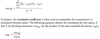
The Pearson correlation coefficient is commonly used to measure the linear relationship between two variables. The Pearson correlation is defined by dividing covariance (cov_XY) by the product of the two assets’ standard deviations (σ_xσ_Y).

ρ_XY = cov_XY / (σ_xσ_Y)

Because many financial variables have nonlinear relationships, the Pearson correlation coefficient is only an approximation of the nonlinear relationship between financial variables. Thus, when applying the Pearson correlation coefficient in financial models, risk managers and investors need to be aware of the following five limitations:

1. The Pearson correlation coefficient measures the linear relationship between two variables, but financial relationships are often nonlinear.
2. A Pearson correlation of zero does not imply independence between the two variables. It simply means there is not a linear relationship between the variables. For example, the parabola relationship defined as Y = X² has a correlation coefficient of zero. There is, however, an obvious nonlinear relationship between variables Y and X.
3. When the joint distribution between variables is not elliptical, linear correlation measures do not have meaningful interpretations. Examples of common elliptical joint distributions are the multivariate normal distribution and the multivariate Student’s t-distribution.
4. The Pearson correlation coefficient requires that the variance calculations of the variables X and Y are finite. In cases where kurtosis is very high, such as the Student’s t-distribution, the variance could be infinite, so the Pearson correlation coefficient would be undefined.
5. The Pearson correlation coefficient is not meaningful if the data is transformed. For example, the correlation coefficient between two variables X and Y will be different than the correlation coefficient between ln(X) and ln(Y).

Question 22

Spearmans Rank Correlation

Answer 22

Ordinal measures are based on the order of elements in data sets. Two examples of ordinal correlation measures are the Spearman rank correlation and the Kendall τ . The Spearman rank correlation is a nonparametric approach because no knowledge of the joint distribution of the variables is necessary. The calculation is based on the relationship of the ranked variables. The following equation defines the Spearman rank correlation coefficient where n is the number of observations for each variable, and d_i is the difference between the ranking for period i.

The Spearman rank correlation coefficient is determined in three steps:

1. Order the set pairs of variables X and Y with respect to the set X.
2. Determine the ranks of X_i and Y_i for each time period i.
3. Calculate the difference of the variable rankings and square the difference.

Question 23

Kendall’s τ

Answer 23

Both Spearman’s rank correlation coefficient and Kendall’s τ are similar to the Pearson correlation coefficient for ranked variables because perfectly correlated variables will have a coefficient of 1.

The Kendall τ will be 1 if variable Y always increases with an increase in variable X. The numerical amount of the increase does not matter for two variables to be perfectly correlated. Therefore, for most cases, the Kendall t and the Spearman rank correlation coefficients will be different.

Question 24

Limitations of Ordinal Risk Measures

Answer 24

Ordinal correlation measures based on ranking (i.e., Spearman’s rank correlation and Kendall’s τ ) are implemented in copula correlation models to analyze the dependence of market prices and counterparty risk. Because ordinal numbers simply show the rank of observations, problems arise when ordinal measures are used for cardinal observations, which show the quantity, number, or value of observations.

• Ordinal correlation measures are less sensitive to outliers, which are extremely important in VaR and stress test models during extreme economic conditions. Numerical values are not important for ordinal correlation measures where only the rankings matter. Thus, since outliers do not change the rankings, ordinal measures underestimate risk by ignoring the impact of outliers.
• Another limitation of Kendalls τ occurs when there are a large number of pairs that are neither concordant nor discordant. In other words, the Kendall τ calculation can be distorted when there are only a few concordant and discordant pairs.

Question 25

Explain the purpose of copula functions and the translation of the copula equation

Answer 25

A correlation copula is created by converting two or more unknown distributions that may have unique shapes and mapping them to a known distribution with well-defined properties, such as the normal distribution. A copula creates a joint probability distribution between two or more variables while maintaining their individual marginal distributions.

A copula function, C, can then be defined as follows:

Question 26

Describe the Gaussian copula

Answer 26

A Gaussian copula maps the marginal distribution of each variable to the standard normal distribution which, by definition, has a mean of zero and a standard deviation of one. The key property of a copula correlation model is preserving the original marginal distributions while defining a correlation between them. The mapping of each variable to the new distribution is done on percentile-to-percentile basis.

Question 27

Time dynamic of PD for non-investment grade companies

Answer 27

Non-investment grade companies have a higher probability of default in the near term during the company crisis state. If the company survives past the near term crisis, the probability of default will go down over time.

Question 28

Correlated default time

Answer 28