Topics 21-23

Question 1

Compare the different ways of representing credit spreads

Answer 1

Question 2

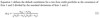
Define and compute the Spread ‘01

Answer 2

DV01 captures the dollar price change from a one basis point change in the
current yield. A similar concept for credit spreads is known as DVCS (i.e., spread ‘01). Here, the potential change in the bond price is estimated from a one basis point change in the z-spread. Specifically, the z-spread is shocked 0.5 basis points up and 0.5 basis points down and the difference is computed.

Intuitively, the smaller the z-spread, the larger the effect on the bond price (i.e., the greater the credit spread sensitivity). This result is straightforward because the same one basis point change represents a larger shock relative to the current z-spread when the z-spread is low. Thus, the DVCS exhibits convexity.

Question 3

Explain how default risk for a single company can be modeled as a Bernoulli trial

Answer 3

A Bernoulli trial is an experiment or process where the outcome can take on only two values: success or failure (the firm does or does not default during a particular time period).

An important property of the Bernoulli distribution is that each trial is conditionally
independent. That is, the probability of default in the next period is independent of
default in any previous period.

Question 4

Explain the relationship between exponential and Poisson distributions

Answer 4

Question 5

# Define the hazard rate and use it to define probability functions for
default time and conditional default probabilities, calculate the conditional default probability given the hazard rate

Answer 5

The hazard rate (i.e., default intensity) is represented by the (constant) parameter λ and the probability of default over the next, small time interval, dt, is λdt.

If the time of the default event is denoted t*, the cumulative default time distribution F{t) represents the probability of default over (0, t):

P(t* < t ) = F(t) = 1 - e^-λt

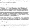
The marginal default probability (or default time density) function as the derivative of F(t) with respect to the variable t:

λe^-λt

It is evident that this quantity is always positive indicating that the probability of default increases over time related to the intensity parameter λ.

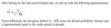
If we examine the probability of default over (t, t + τ) given survival up to time t, the function is a conditional default probability. The instantaneous conditional default probability (for small τ) is equal to λτ.

The conditional one-year probability of default, assuming survival during the first year, is equal to the difference between the unconditional two-year PD and the unconditional oneyear PD, divided by the one-year survival probability.

Question 6

Calculate risk-neutral default rates from spreads

Answer 6

Question 7

Describe advantages of using the CDS market to estimate hazard rates

Answer 7

The primary advantage of using CDS to estimate hazard rates is that CDS spreads are observable.

We can draw on the logic of a reduced form model to use the observable, liquid CDS to infer the estimates of the hazard rate.

Liquid contracts exist for several maturities (e.g., 1, 3, 5, 7 and 10 years are common). Furthermore, a large number of liquid CDS curves are available (800 in U.S. markets, 1,200 in international markets) and the contracts are more liquid than the underlying cash bonds (i.e., narrower spreads and more volume).

Question 8

Explain how a CDS spread can be used to derive a hazard rate curve

Answer 8

• The CDS spreads provide several discrete maturities to extract hazard rates.
• Technically, hazard rates are measured every instant in time so the CDS data will only provide a few observable data points and will require some form of interpolation or piecewise construction to complete the curve.
• The fact that the CDS swap spread is observable allows for the inference of default probability for the 1-year maturity by equating (PV of expected payments in default) and (PV of expected premiums paid). Thus, given an assumed recovery rate (usually 40%), the probability of default and, hence, the hazard rate can be inferred for the first period (using the first piecewise portion of the earlier hazard function).
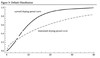
• The bootstrapping procedure is then employed so that the hazard rate for the first period is used to infer the hazard rate for the second period from the piecewise function (using the observable information from the second CDS contract with a 3-year maturity, a recovery rate assumption, and the swap curve). Similarly, the hazard rate from the second period is an input to find the hazard in the third period, and so on. In this fashion, a graph can be constructed showing the CDS spreads, hazard rates, and default density.

Question 9

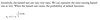
Explain how the default distribution is affected by the sloping of the spread curve

Answer 9

As a benchmark, consider the impact of spreads that are constant for all maturities, that is, the market’s expectations for default is constant. In this case, the spread curve would be flat implying the probability of defaulting in the near term is the same as defaulting in the long run.

The most common spread curve is upward sloping. Thus, the aggregate market forecast is that default is unlikely in the near term but increases with the forecast period. In contrast, spread curves, although unusual, may be downward sloping. This phenomenon would indicate relatively high expectations of short-term default (distress) but, if the firm can right itself, it will likely survive for a sufficiently long period of time.

Question 10

Define spread risk and its measurement using the mark-to-market and spread volatility

Answer 10

To measure spread risk, the mark-to-market of a CDS and spread volatility can be used. The mark-to-market effect is computed by shocking the entire CDS curve up and down by 0.5 basis points (similar to spread ‘01). Note the slight difference from spread ‘01 where the z-spread, a single value, was shocked. Thus, the entire CDS curve moves up and down by a parallel amount.

An alternative measure of spread risk is to compute the volatility (standard deviation) of spreads. The spread volatility can use historical data or can be forward-looking based on a subjective probability distribution. Not surprisingly, the spread volatility spiked extremely high during the recent financial crisis for many financial services firms.

Question 11

Define and calculate default correlation for credit portfolios

Answer 11

Default correlation measures the probability of multiple defaults for a credit portfolio issued by multiple obligors.

! Default correlation has a tremendous impact on portfolio risk. But it affects the volatility and extreme quantiles of loss rather than the expected loss

Question 12

Identify drawbacks in using the correlation-based credit portfolio framework

Answer 12

A major drawback of using the default correlation-based credit portfolio framework is the number of required calculations - the number of pairwise correlations is equal to n(n — 1).

In addition, certain characteristics of credit positions do not fit well in the default
correlation credit portfolio model. For example, credit default swap (CDS) basis trades may not be modeled simply by credit or market risk.

Additional drawbacks in using the default correlation-based credit portfolio framework are related to the limited data for estimating defaults.

Question 13

Assess the impact of correlation on a credit portfolio and its Credit VaR. Define and calculate Credit VaR

Answer 13

The effects of default, default correlation, and loss given default are important determinants in measuring credit portfolio risk. A portfolio’s credit value at risk (credit VaR) is defined as the quantile of the credit loss less the expected loss of the portfolio. Default correlation impacts the volatility and extreme quantiles of loss rather than the expected loss. Thus, default correlation affects a portfolio’s credit VaR.

The term “granular” refers to reducing the weight of each credit as a proportion of the total portfolio by increasing the number of credits. As a credit portfolio becomes more granular, the credit VaR decreases. However, when the default probability is low, the credit VaR is not impacted as much when the portfolio becomes more granular.

Question 14

Describe the use of a single factor model to measure portfolio credit risk, including the impact of correlation

Answer 14

An important property of the single-factor model is conditional independence.

Conditional independence states that once asset returns for the market are realized, default risks are independent of each other. This is due to the assumption for the single-factor model that return and risk of assets are correlated only with the market factor. The property of conditional independence makes the single-factor model useful in estimating portfolio credit risk.

Question 15

Conditional Default Distribution Variance

Answer 15

Question 16

Credit VaR with a Single-Factor Model

Answer 16

The unconditional distribution used to calculate credit VaR is determined by the following steps:

Question 17

Describe how Credit VaR can be calculated using a simulation of joint defaults

Answer 17

The following four steps are used to compute a credit VaR under the copula methodology:

1. Define the copula function.
2. Simulate default times.
3. Obtain market values and profit and loss data for each scenario using the simulated default times.
4. Compute portfolio distribution statistics by adding the simulated terminal value results.

Question 18

Covered bonds

Answer 18

Covered bonds are on-balance sheet securitizations. A pool of mortgages, which secure a bond issue, is separated from other loans into a covered pool on the originator’s balance sheet. Investors have higher priority than general creditors if a bank defaults. Principal and interest is paid and guaranteed by the originator and is not based on the performance of the underlying assets themselves. Thus, covered bonds are not true securitizations since the assets are not part of a bankruptcy-remote structure and the investors have recourse against the originator.

Question 19

Mortgage pass-through securities

Answer 19

In contrast to covered bonds, mortgage pass-through securities are true off-balance sheet securitizations. Investors receive cash flows based entirely on the performance of the pool less associated fees paid to the servicer. Most pass-throughs are agency mortgage-backed securities (MBS) that carry implicit or explicit government guarantee of performance. Thus, default risk is not a serious concern. The primary risk is due to prepayment of principal by the homeowner, most likely from refinancing after interest rate declines or home sales.

Question 20

Collateralized mortgage obligations (CMOs)

Answer 20

CMOs are MBSs that tranche (i.e., divide) cash flows into different securities based on predetermined conditions. The resulting tranches can have long or short maturities, fixed or floating cash flows, or other varieties and conditions.

The most basic structure is the waterfall or sequential pay structure where Tranche 1 receives all principal and its portion of interest in each period until it is paid off. The remaining tranches will receive interest only until Tranche 1 is retired and then principal will flow down to Tranche 2, and so on. Not surprisingly, Tranche 1 will have a very low prepayment risk as it expects to receive all principal payments before other bondholders.

Question 21

Structured credit products

Answer 21

Like other structured products, this pool of assets is backed by risky debt instruments. The difference is that structured credit products create tranches that have different amounts of credit risk.

• The most junior (i.e., equity) tranches bear the first losses and are most likely to be written down from defaulted assets. If the equity tranche is completely wiped out, the next most junior tranche will bear the credit risk of subsequent defaults.
• The most senior tranche will have the highest credit rating and the lowest probability of writedowns.

Question 22

Asset-backed securities

Answer 22

This is the most general class of securitizations where cash-flow generating assets are pooled and subsequently tranched. Under this definition, MBS is a special case of the more general ABS. Other varieties include collateralized bond obligations (CBO), collateralized debt obligations (CDO), collateralized loan obligations (CLO), and collateralized mortgage obligations (CMO). There exist even more complex securities that pool other securitizations together such as CDO-squared (CDO of CD Os).

Question 23

Describe tranching and the distribution of credit losses in a securitization

Answer 23

• The capital structure of a securitization refers to the priority assigned to the different tranches. In general, the most senior tranches at the top of the capital structure will have the highest priority to receive principal and interest. Since these securities are perceived to be the safest, they also receive the lowest coupon.
• The equity tranche is the slice of the cash flow distribution with the lowest priority and will absorb the first losses up to a prespecified level. These securities typically do not carry a fixed coupon but receive the residual cash flows only after the other security claims are satisfied. Therefore, the return is variable and, hence, the term “equity.” Typically, the equity tranche is the smallest part of the capital structure.
• Between the senior and equity tranches is the mezzanine tranche (i.e., the junior tranche). The mezzanine tranches will absorb losses only after the equity tranche is completely written down. To keep the securitization viable, the mezzanine tranches will be purposefully thin.

Question 24

Credit enhancement

Answer 24

In general, credit enhancement can be divided into internal and external credit enhancement mechanisms.

• The term external credit enhancement means that the credit protection takes the form of insurance or wraps purchased from a third party, typically a monoline insurer.
• Two examples of internal credit enhancements are overcollateralization and excess spread.
  
  • Overcollateralization is when the pool offers claims for less than the amount of the collateral. For example, consider a collateralized MBS with 101 mortgages in the collateral pool, but the face value of the bonds across all tranches only totals 100 mortgages. Overcollateralization is a hard credit enhancement because the protection is available at the origination of the pool.
  • The excess spread is the difference between the cash flows collected and the payments made to all bondholders. For example, if the weighted average of the collateral is 8% (net of fees) and the weighted average of the payments promised to the senior, junior, and equity tranches is 7%, then the residual 1% accumulates in a separate trust account. The excess spread will be invested and is available to make up future shortfalls. Since the excess spread is zero at origination, it is considered a soft credit enhancement.

Question 25

Describe a waterfall structure in a securitization

Answer 25

A waterfall structure outlines the rules and conditions that govern the distribution of collateral cash flows to different tranches. In the simplest example of a securitization, the senior and junior bonds will receive their promised coupons conditional on a sufficient amount of cash inflows from the underlying loans. The residual cash flow, if any, is called the excess spread. The overcollateralization triggers will decide how the excess is divided between the equity investors and the accumulating trust. Intuitively, the underlying cash flows will be largest in the earlier periods so the trust will build up a reserve against future shortfalls.

In practice, this process can be quite complex as there may be a dozen tranches or more with different coupons, maturities, and overcollateralization triggers. The waterfall is further complicated by loan defaults. A simplifying assumption would incorporate a constant default rate which can be built into the waterfall distribution. As the loans mature, the actual incidence of the loan defaults will increase or decrease the value of the respective tranches.

Question 26

Identify the key participants in the securitization process, and describe conflicts of interest that can arise in the process

Answer 26

• The nature of the securitization process from original loan to tranche issuance necessarily involves many different participants. The first step begins with the originator who funds the loan. The originator may be a bank, mortgage lender, or other financial intermediary. The term “sponsor” may be used if the originator supplies most of the collateral for the issue.
• The underwriter performs a function similar to the issuance of traditional debt and equity. The underwriter structures the issue (i.e., engineers the tranche size, coupon, and triggers, and sells the bonds to investors). The underwriter warehouses the collateral and faces the risks that the issue will not be marketed or that the collateral value will drop.
• The credit rating agencies (CRAs) are an important part of the securitization process. Without their explicit approval via credit ratings, investors would be at a severe disadvantage to assess the riskiness of the issue. The credit rating agencies can influence the size of the tranches by selecting the attachment points and thus are active participants in the process. In addition, the CRAs may influence the issue by requiring enhancements. There is a natural conflict of interest because the CRAs want to generate profit and grow their business, but it may come at the expense of allocating larger portions of the capital structure to lower iterest paying senior notes. Investors can alleviate this concern by performing their own (costly) analysis or purchasing a wrap or insurance against the issue.
• The role of the servicer is multifaceted and possibly understated. The servicer must collect and distribute the collateral cash flows and the associated fees. In addition, the servicer may need to provide liquidity if payments are late and resolve default situations. It is not hard to envision the conflict of interest in foreclosure: the servicer would, all else equal, like to delay foreclosure to increase their fees, while investors want as quick of a resolution as possible to minimize the damage and/or lack of maintenance from the homeowners who have no economic incentive to maintain the property.
• When the pool is actively managed, another source of conflict arises. The manager naturally would like to minimize their effort to continually monitor the credit quality of the collateral unless there is a clear incentive to do so. A common feature of securitized pools is for the originator and/or manager to bear the first loss in the capital structure.
• Custodians and trustees play an administrative role verifying documents, disbursing funds, and transferring funds between accounts.

Question 27

Describe a simulation approach to calculating credit losses for different tranches in a securitization

Answer 27

Step 1: Estimate the parameters.

The first step is to estimate the critical parameters, default intensity, and pairwise correlations. The default intensity can be estimated using market spread data to infer the hazard rate across various maturities.

Estimating the correlation coefficients is more challenging because of a lack of usable market data. The copula correlation could be useful in theory but suffers empirical precision in practice. Instead, a sensitivity analysis is performed for various default and correlation pairs.

Step 2 : Generate default time simulations.

The second step identifies if and when the security defaults. Simulation provides information on the timing for each hypothetical outcome.

Step 3 : Compute portfolio credit losses.

The third step uses the simulation output to determine the frequency and timing of credit losses. The credit losses can be “lined up” to assess the impact on the capital structure losses. The tail of the distribution will identify the credit VaR for each tranche in the securitization.

Question 28

Explain how the default probabilities affect the credit risk in a securitization

Answer 28

• It is straightforward to see that, for a given correlation, increasing the probability of default will negatively impact the cash flows and, thus, the values of all tranches.
• Convexity is also an issue for default rates. For equity investors, as default rates increase from low levels, the equity tranche values decrease rapidly then moderately (a characteristic of positive convexity). Since the equity tranche is thin, small changes in default rates will disproportionately impact bond prices at first. Similarly, senior tranches exhibit negative convexity. As defaults increase, the decline in bond prices increases. As usual, the mezzanine impact is somewhere in between: negative convexity at low default rates, positive convexity at high default rates.
• Increasing default probability, while holding correlation constant, generally decreases the VaR for the equity tranches (less variation in returns) and increases the VaR for the senior tranches (more variation in returns). As usual, the mezzanine effect is mixed: VaR increases at low correlation levels (like senior bonds) then decreases at high correlation levels (like equity). These results are summarized in Figure 3.
• As the default correlation approaches one, the equity VaR increases steadily. The interpretation is that although the mean return is increasing so is the risk as the returns are more variable (large losses or very small losses).

Question 29

Explain how default correlations affect the credit risk in a securitization.

Answer 29

• The effect of changing the correlation is more subtle. Consider the stylized case where the correlation is very low, say zero, so loan performance is independent. Therefore, in a large portfolio, it is virtually impossible for none of the loans to default and it is equally unlikely that there will be a large number of defaults. Rather, the number of defaults should be very close to the probability of default times the number of loans. So, the pool would experience a level of defaults very close to its mathematical expectation and is unlikely to impair the senior tranches. Now, if the correlation increases, the default of one credit increases the likelihood of another default. Thus, increasing correlation decreases the value of senior tranches as the pool is now more likely to suffer extreme losses. This effect is exacerbated with a higher default probability.
• Now consider the equity tranche. Recall that the equity tranche suffers the first writedowns in the pool. Therefore, a low correlation implies a predictable, but positive, number of defaults. In turn, the equity tranche will assuredly suffer writedowns. On the other hand, if the correlation increases, the behavior of the pool is more extreme, and there may be high levels of related losses or there may be very few loan losses. In sum, the equity tranche increases in value from increasing correlation as the possibility of zero (or few) credit losses increases from the high correlation.
• The correlation effect on the mezzanine tranche is more complex. When default rates are low, increasing the correlation increases the likelihood of losses to the junior bonds (similar to senior bonds). However, when default rates are relatively high, increasing the correlation actually decreases the expected losses to mezzanine bonds as the possibility of few defaults is now more likely. Accordingly, the mezzanine bond mimics the return pattern of the equity tranche. In short, increasing correlation at low default rates decreases mezzanine bond values, but at high default rates it will increase mezzanine bond values.
• Increasing correlation decreases senior bond prices as the
  subordination is more likely to be breached if defaults do indeed cluster. In contrast, equity returns increase as the low default scenario is more probable relative to low correlation
  where defaults are almost certain
• The senior VaR also increases consistently with correlation. If correlation is low and default frequency is relatively high, then senior bonds are well insulated. In fact, at the 10% subordination level, the senior bonds would be unaffected even at a high default rate. At the other extreme, when correlations are high (0.6 or above), then the VaRs are quite similar regardless of the default probability. Hence, generally speaking, correlation is a more important risk factor than default probability which may not be entirely intuitive.
• The implications for the mezzanine tranche are, again, mixed. When default rates and correlations are lower, the mezzanine tranche behaves more like senior notes with low VaRs.
  However, when the default probabilities are higher and/or pairwise correlation is high, the risk profile more closely resembles the equity tranche. These results are summarized in Figure 4.

Question 30

Explain how default sensitivities for tranches are measured

Answer 30

Question 31

Describe risk factors that impact structured products

Answer 31

There are at least three other risks that deserve discussion: systematic risk, tranche thinness, and loan granularity.

• Similar to a well-diversified equity portfolio that cannot eliminate systematic risk, the same holds true for credit portfolios. Unfortunately, even when the collateral pool is well-diversified among lenders, terms, geography, and other factors, high systematic risk expressed in high correlations can still severely damage a portfolio. As previously discussed, with increases in pairwise correlations, the likelihood of senior tranche writedowns increases as well.
• The equity and mezzanine tranches are relatively thin. This also manifests itself in the relative closeness of the 93% and 99% credit VaR. The implication is that given that the tranche has been breached, the loss is likely very large.
• Loan granularity references the loan level diversification. For example, in a collateralized MBS pool, the portfolio composition is a few loans but the loans are of substantial size. This reduction in sample size increases the probability of tail events in relation to an equal sized portfolio constructed with more loans of smaller amounts.

Question 32

Define implied correlation and describe how it can be measured

Answer 32

The implied correlation is a very similar concept to the implied volatility of an equity option. Starting with observed market prices
and a pricing function for the tranches, it is possible to back out the unique implied correlation to calibrate the model price with the market price.

The mechanical part of the process involves several intermediate steps. First, the observable credit default swap (CDS) term structure is used to extract risk-neutral default probabilities
and possibly recovery rates. Assuming constant pairwise correlation and market prices for the respective tranches, the default estimates and correlation estimates can be fed into a
copula. The output is the risk-neutral implied correlation (i.e., base correlation) per tranche. The correlation estimates will vary between the tranches and are not likely to be constant giving rise to correlation skew.

Question 33

Identify the motivations for using structured credit products

Answer 33

• Loan originators, who help create securitizations by selling loans into a trust, are attracted to borrowing via securitization given its ability to provide a lower cost of funding. Without securitization, loans would either be retained or sold in the secondary market. These alternatives would likely be more costly than securing funding via securitization. A lower cost of funding can be obtained given the diversification of the loan pool and the reputation of the originator for underwriting high-quality loans. However, some loan pools, such as commercial mortgage pools, can be difficult to diversify. Thus, an element of systematic risk may still exist, which could lead to an underestimation of overall risk. An additional benefit of securitization for loan originators is the collection of servicing fees.
• Investors, who purchase the assets in a securitization, are attracted to investing in diversified loan pools that they would not otherwise have access to without securitization, such as mortgage loans and auto loans. In addition, the ability to select a desired risk-return level via tranching offers another advantage for investors. Equity tranches will offer higher risk-return levels, while senior tranches will offer lower risk-return levels. However, it is important for investors to conduct the proper due diligence when analyzing potential tranche investments in order to understand the actual level of risk involved.

Question 34

Hazard rate

Answer 34

Cumulutive default time distribution (probabilty of default in time t):

p(t) = 1 - e^-λt

Survival time distribution:

p(t) = e^-λt

Poisson distribution:

p(x) = (λ^xe^-λ)/x!

• x - number of deafult events within the set time

The conditional default probability over short interval (t, t + Δ) is given by λΔ; this is the definition of the hazard rate. i.e., the conditional default probability = instantaneous hazard rate = F’(t)Δ/[1 - F(t)] = [λ*exp(-λ*t)]Δ/exp(-λ*t) = λΔ