chapter 3: normal distribution

Question 1

While a histogram is a great way to get an overview of data, it can be restrictive when we must…

Answer 1

…establish the sizes of our bins and the placement of their endpoints

Question 2

If our bins are initially positioned non-optimally or our bin sizes are too large…

Answer 2

…we can easily get a misleading graph

Question 3

μ

Answer 3

Mu. The mean of a density curve (and a normal distribution, which is also the center of gravity for the curve. You could therefore put a see-saw point at the mean. On a skewed curve, the mean moves out toward the tail, in the direction of the skewness.

Question 4

σ

Answer 4

lower case sigma. the standard deviation of a normal distribution

Question 5

normal distribution

Answer 5

a continuous bell shaped symmetrical distribution

Question 6

You write out a normal distribution with mean μ 10 and s.d. (standard deviation) σ 2 (pictured) as…

Answer 6

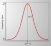
N(10,2)

Question 7

P ( μ - σ < Y < μ + σ) = 0.68

Answer 7

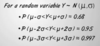
probabilities that a result will fall within 1x, 2x, or 3x of the standard deviation in a normal distribution

Question 8

changing the σ standard deviation in a normal distribution curve results in the curve itself becoming either…

Answer 8

short and fat or tall and narrow

Question 9

68 - 95 - 99.7 rule

aka the imperical rule

Answer 9

1. 68% with be within μ ± σ
2. 95% will be within μ ± 2σ
3. 99.7% will be within μ ± 3σ

Question 10

z-score

or standardized value

Answer 10

The number of deviations ( σ ) a data point is awa from its mean ( μ ). In other words, if the point 𝑥 has area 𝐴 to the left of it under 𝑁(μ,𝜎), then the adjusted value 𝑧 will have area 𝐴 to the left of it under 𝑁(0,1)

Question 11

Ultimately (if we keep making more observations and decreasing our bin sizes)…

Answer 11

…this process gives us a smooth curve.

Question 12

A density curve always has these to properties

Answer 12

1. It is always on or above the horizontal (x) axis.
2. It has area of exactly 1 beneath it.

Question 13

Knowing that a certain variable has a distribution best described by a density curve in a certain population allows us to…

Answer 13

…say things about the proportions of individuals in that population that exhibit certain values

Question 14

uniform distribution

Answer 14

A type of distribution in which each value is just as likely to occur anyywhere along it.

Question 15

The mode of a density curve

Answer 15

the value which occurs most often, or the value beneath the highest point of a density curve (the peak).

Question 16

Standard Normal Distribution

Answer 16

𝑁(0,1)

this allows us to make a representative normal disribution for all others.

Question 17

Standard Normal Table

Answer 17

A list of several hundred values in a reference chart of areas for a normal distribution density curve for easy reference. Suppose that we’d like to know the percentage of area under the curve 𝑁(0,1) to the left of the point -1.52. We would look on the Standard Normal Table for the “-1.5” in the left-hand column and at the row to the right of it. We would then look for the entry underneath the number “.02” in the top row, and we would find “.0643”. If we wish to find the proportion of observations greater than a given value, we simply subtract the value that we find in the table from 1, since 1 is the total area.

Question 18

cumulative proportion

Answer 18

in a distribution is the proportion of observations in the distribution that are less than or equal to x.

Question 19

Using Table A to Find Normal Proportions

Answer 19

Step 1. State the problem in terms of the observed variable x. Draw a picture that shows the proportion you want in terms of cumulative proportions.

Step 2. Standardize x to restate the problem in terms of a standard Normal variable z.

Step 3. Use Table A to find areas to the left of z. The fact that the total area under the curve is 1 may also be necessary to find the required area.