Biodiversity

Question 1

Diversity (types)

Answer 1

Genetic diversity
Species diversity
Ecological diversity
Functional diversity

Question 2

Biodiversity movement

Answer 2

Movement addressing environmental concerns in relation to politics, biology, and ethics

Question 3

Ecological diversity

Answer 3

Concept relating to variability of trophic levels, life cycles, and biological resources

Question 4

Biodiversity

Answer 4

Term analogous to biological diversity; popularized in the 80s by E.O. Wilson

Question 5

Biological diversity

Answer 5

Concept referring to the variety and abundance of species in a spatial unit

Question 6

Taxonomic distinctness

Answer 6

Measure of diversity similar to Simpson’s index

Question 7

Diversity measures

Answer 7

Measure taking into account richness and abundance

Question 8

Richness

Answer 8

Simply the number of species in a spatial unit

Question 9

Evenness

Answer 9

Measure of differences in abundance between species

Question 10

Diversity index

Answer 10

A single statistic conveying information on richness and abundance

Question 11

Heterogeneity

Answer 11

Concept incorporating both richness and evenness

Question 12

a-diversity

Answer 12

Diversity within a defined spatial area

Question 13

b-diversity (concept)

Answer 13

The extent to which the diversity of two or more spatial units differ; Concept conceived by Whittaker (1960) originally to measure diversity changes between samples along transects, but commonly used for changes along other spatial arrangements and over time.

Question 14

Dominance

Answer 14

The extent to which one or a few species are primarily conform a community

Question 15

Abundance (and evenness) visualization

Answer 15

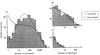
1) Histogram: abundance (y axis) against ranked species (x axis)
2) Rank/abundance plot (aka Whittaker): line graph of relative abundance (in log₁₀ scale) against ranked species; the steeper the curve, the lower the evenness of the assemblage
3) k-dominance plot: line graph of cumulative relative abundance (y) against ranked species (x); The more elevated the line is from the x axis, the less diverse diverse the assemblage
4) Abundance/biomass comparison (ABC plot): Same as k-dominance, but cumulative relative biomass also plotted
5) Fisher plot: Number of species (y) plotted against number of individuals (x); looks like a very lef-skewed histogram
6) Preston plot: Number of species (y) plotted against number of individuals in a log₂ scale arranged in “octaves” (x); can use other log base; looks like a bell-shape (i.e., log normal model)

Question 16

Pattern vs process

Answer 16

Pattern refers to the way a system behaves
Process refers to the reasons why a system behaves in a particular way

Question 17

Biodiversity measurement (assumptions)

Answer 17

1. All species are equal
2. All individuals are equal
3. Abundance is expressed in comparable units

Question 18

Biodiversity (nature as a science)

Answer 18

Biodiversity is a comparative science by nature

Question 19

Community

Answer 19

Group of organisms in a defined area that interact among themselves

Question 20

Guild

Answer 20

A group of organisms using the same resources

Question 21

Assemblage

Answer 21

Group of organisms in a communiy that share a certain phylogeny

Question 22

Local guild

Answer 22

Group of organisms using the same resources and co-ocurring in an area

Question 23

Ensemble

Answer 23

Group of organisms sharing geographic distribution, resources, and phylogeny

Question 24

Self-similarity

Answer 24

A pattern of diversity maintained across different spatial scales

Question 25

Geographic boundary of a community

Answer 25

Set arbitrarily by te researcher

Question 26

Statistical vs biological models

Answer 26

Statistical models aim to describe observed patterns, while bioloical models aim to explain those patterns

Question 27

Logarithmic series model

Answer 27

Statistical model proposed by Fisher (1940s) to describe the relationship between number of species and number of individuals in those species;

αx, αx²/2, αx³/3…αx/n

αx is the number of species predicted to have one individual, and so on

the paremeter α is a good index of diversity

Question 28

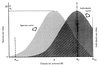
Log normal model

Answer 28

Statistical model proposed by Preston (1940s); Describes species abundance against species ranks (log₂) resulting in classes called octaves. Can use other bases (e.g., 3 or 10).

Most large assemblages follow this distribution.

Incroporates γ as an additional parameter when a number of individuals curve is superimposed on the number of species curve.

The distribution is canonical when γ=1, in which case the mode of the individuals curve coincides with the upper tail of the species curve.

Question 29

Log normal: Statistical explanation for its commonness in real data

Answer 29

Log normal distribution might be common as a result of the central limit theorem, wich states that when the amount of a variable is determined by a large number of factors, random variation in the factors will result in a normal distribution.

Additional support: more specious assemblages tend to be canonicl compared to less specious

Question 30

Log normal: Biological explanation for its commonness in real data

Answer 30

Log normal distribution can be a consequence of random niche division/invasion.

Question 31

Log normal distribution: Veil line

Answer 31

Truncation point of a log normal curve resulting as a consequence of difficulty sampling the less abundant species.

Note that veiled distributions are more difficult to fit.

Question 32

Log normal (fitting and nature of data)

Answer 32

Technically, a log normal distribution should only be fitted to continuous abundance data such as biodiversity, but large discrete datasets work fine because they often act as continuous

Question 33

Poisson log normal

Answer 33

A variation of the log normal distribution that assumes discrete abundance classes.
Uses the Poisson parameter λ, which is also a robust index of diversity.

Question 34

Log normal: visual method for seeing fit of data

Answer 34

Plotting cumulative frequency of species (y) against log₂ rank classes (x) should look like a straight line

Question 35

Log normal: implication of departure

Answer 35

Departure of an assemblage from a log normal distribution is often used as a sign of environmental disturbance (though this is a challenged view)

Question 36

Overlapping distributions (explain)

Answer 36

Data are often described by more than one distribution model

Question 37

Overlapping of log series and log normal distribution

Answer 37

Potentially explained by a difference between permanent species (log normal distribution) and occasional species (log series distribution); when plotted together, the result is a left-skewed distribution.

Question 38

Other statistical models besides log series and log normal

Answer 38

Negative binomial; Zipf-Mandelbrot

Question 39

Fitting a model to data

Answer 39

Goodness of fit tests (usually X²) are used to evaluate the relationship between observed and expected frequencies.

X² = [(observed - expeted)²/expected]

A P<0.05 means the model does not describe the observed pattern.

Question 40

Goodnes of fit test for small datasets

Answer 40

Kolmogorov-Smirnov goodness of fit test may be applied to small datasets and can also be used to compare two datasets

Question 41

Niche appointment models

Answer 41

Noche appintmt models are based on the assumption that a community has a property called niche space that is divided in a certain way among species.

Different biological models vary in the way they propose niche fragmentation/filling occurs.

Question 42

Niche filling

Answer 42

An alternative mehcanism to niche fragmentation in which additional niche space is accomodated (e.g., newly formed habitats like island and lakes).

Question 43

Deterministic vs stochastic statistical diversity models

Answer 43

Deterministic models assume tat a set number of individuals, N, will be distributed among species, S, in a particular way.

Stochastic models establish that replicated communities will vary in their species abundances.

Most statistical models are deterministic, while most biological models are stochastic

Question 44

Geometric series model

Answer 44

The geometric series is a biological model that assumes dominance-based niche appointment undrer limiting factors, and a relationship between allocated niche and abundance.

Usually observed in data from species-poor and harsh environments.

Question 45

Broken stick model

Answer 45

Biological model proposed by McArthur (late 1950’s). The model proposes niche division occurs like a stick is simultaniously being divided at random. Imporant in the development of ecological thought but rarely fits empirical data.

Question 46

Tokeshi’s models

Answer 46

Niche appointment models (biological models) proposed by Tokeshi (90’s). They all assume niche space is occupied by species proportionally to abundance, but propose different mechanisms of niche division.

1) Dominance pre-emption: niche of least abundant species is subdivided
2) Random fracion: niche to be subdivided is selected at random
3) Power fraction: probabiltiy of division is moslty random but slighlty influenced by size
4) McArthur fraction model: probability of division proportional to size
5) Dominance decay: largest niche invariably split
6) Random assortment: No relationship between niche appointment and species abundance
7) Composite: small niches divided randomly and large niches divided following a rule

Question 47

Caswell’s neutral model

Answer 47

An alternative biological model, proposed by Caswell (late 1970’s). Operates by examining how species abundance would occur in a community if all interactions were removed.

Question 48

Hubbell’s neutral theory of biodiversity and biogeography

Answer 48

A more ambitious neutral model than Caswell’s. Proposed y Hubbel (2000). In this bioloical model, metacommunities are composed of a set of local communities that are always saturated, so there is no place for new individuals until others die.

The relative abundance of a species in a local community is dictated by its aundance in the metacommunity.

Explains a great number of empirical systems. One complication is that it requires simulations.

Question 49

Fitting stochastic niche appointment models to empirical data

Answer 49

Communities are repetedly constructed using simulation, which allows to produce confidence limits on expected abundances. If the observed model fits within the confidence intervals, a model is said to fit the data.

Does not work if the variance is greater than that predicted.
Replication of observations in required (increases power) but not necessary (i.e., when detecting community changes over time).

Question 50

Comparing abundance patterns between communities

Answer 50

The Kolmogorov-Sminrov two-sample test allows to determine whether two communities have the same pattern of abundance.

Question 51

Criteria for classifying species as rare

Answer 51

1) Relative criteria: Example: species in the first quartile of the distribution are considered rare. This will vary depending on the measure used to quantify abundance (e.g., number of individuals vs biomass).
2) Absolute criteria: Example, all species with only one individual (singletons) are considered rare.

Question 52

Rarity (mechanistic components)

Answer 52

Rarity occurs as a function of:
geograhpic distribution, habitat specificity, and local population size.

Question 53

Rarity (definition according to the International Union for Conservation of Nature and Natural Resources

Answer 53

Taxa with small populations and restricted geographic areas that are often scattered.

Question 54

Biggest obstacles for measuring biodiversity

Answer 54

1. The variety of species conepts and lack of consensus
2. Taxonomic bias
3. Sampling issues (rare = lower detectability); sampling scale (spatial and temporal); sampling effort

Question 55

Morphospecies (aka morphotypes)

Answer 55

Morphospecies are taxa that are distinguishable on a morphological basis, without necessary taxonomic knowledge.

Question 56

Ways of expressing richness measures

Answer 56

1. Numerical (i.e., number of species per abundance or biomass category)
2. Species density (number of species per area unit)
3. Incidence (number of sample units in which a species is present)

Question 57

Richness indices

Answer 57

Richness indices attempt to compensate for sampling effects by dividing S by N in some way. Examples include Margalef’s diversity index and Menhinick’s index. These indeces are still influenced by sampling effort.

Question 58

Methods to estimate true richness from samples

Answer 58

1) Extrapolation
2) Examining shape of species abundane curves
3) Nonparametric estimators (most powerful approach)

Question 59

Species accumulation curves

Answer 59

Examines the rate at which new species are added by simulating the the samples in a randomized way a certain number of times. Mean and SD are also calculated.

The product is a plot of cumulative numer of species (y) by sampling effort (x).

Species accumulation curves produce total values of richness.
Can be used to 1) compre communities
2) evaluate sample size adequacy.

Question 60

Species area curves

Answer 60

Similar to species accumulation curves, examines the rate at which new species are added to an inventory, but uses area units instead of sequential sampling. Widely used in botanical surveys.

Question 61

Rarefaction curves

Answer 61

Rarefaction curves are similar to species accumulation curves, but instead of explaining richness as samples are added, it explains it by examining what pattern would have been produced if sampling effort had been reduced.

Rarefaction curves produce mean values of richness and can be viewed as the statistical product of a species accumulation curve.

Rarefaction curves are mostly used to compare assemblages.

Question 62

Richness extrapolation (conditions)

Answer 62

To extrapolate richness, sampling needs to:

1) occur in a systematic way as opposed to ad hoc (as needed)
2) occur in a homogenous habitat

Question 63

Richness extrapolation (types)

Answer 63

Functions of richness extrapolation can be:

1) asymptotic (e.g., negaive exponential, Michaelis-Menten equation)
2) nonasymptotic (e.g., log linear models)

Question 64

Abundification

Answer 64

A parametric method to estimate the overall species richness in an assemblage or the increase in S expected from additional sampling.

α is estimated from the observed S and N, and used to deduce S given a larger N.

Requires that the data conform to a log series distribution.

Also allows to compare communities with unequal sampling effort.

Question 65

Log normal: Issues for fitting to data

Answer 65

1) assumes continuous data
2) requires a large sample size (N > 1,000)
3) choosing abundance classes is problematic
4) no method for condifence intervals
5) Poisson log normal is harder to fit

Question 66

Nonparametric estimators of richness

Answer 66

Not based on any particular species abundance model and therefore avoid issued related to fitting parametric models.

Question 67

Chao 1

Answer 67

Chao 1 is a nonparametric estimator for absoule richness based on a ratio between singletons and doubletons:

S_Chao1 = S_obs + (F₁²/2F₂)

• F*₁: number of singletons
• F*₂: number of doubletons

Chao 1 assumes homogeneity among samples.

Question 68

Chao 2

Answer 68

Nonparametric estimator of richness. Variation of Chao 1 for presence/absence data:

S_Chao1 = S_obs + (Q₁²/2Q2)

• Q*₁: species present in only 1 sample
• Q*_2: species present in 2 samples

Question 69

Coverage estimators

Answer 69

Based on the idea that abundant species are likely to be included in any sample and thus provide little information about a community. In constrast, information about rare species is more useful.

Question 70

Abundance-based coverage estimator (ACE)

Answer 70

A coverage estimator based on species with 1 - 10 individuals.

Question 71

Incidence-based coverage estimator (ICE)

Answer 71

A coverage estimator based on species found in ≤10 samples.

Question 72

Other nonparametric estimators

Answer 72

Jacknife 1: uses the numbr of species found that occur one sample.

Jacknife 2: uses the numbr of species found that occur in one and two samples.

Bootstrap estimator: also uses incidence data.

Question 73

Stopping rule

Answer 73

Stopping rule is an indicator that further sampling is not required.

Two examples of approaches to determine the sampling stopping point:

1) Empirical species accumulation curve crosses curve generated by Michealis-Menten.
2) No singletons are left.
3) Subdivide sample in two (at random) and check that both subsamples follow the same pattern.
4) Estimators become stable and stop rising.

Question 74

Richness estimators: desirable qualities

Answer 74

1) can use a sample size as small as posible.
2) Accuracy
3) allow an estimation of variance
4) not biased
5) computationally efficient

Question 75

Species surrogacy tpes

Answer 75

1) Cross-taxon: richness of one taxon used to infer richness of another
2) Within-taxon: familiar or generic richness used as a surrogate for species richness
3) Environmenal: relatonships between environmenal factors and species richness

Question 76

Heterogeneity measures (categories)

Answer 76

Heterogeneity measures are classified as parametric or nonparametric

Question 77

α

Answer 77

Parametric measure of the log series model used to fit the distribution; Can be used as a measure of diversity even when the log series model doesn’t fit the data; It is possible to attach confidence intervals; It’s unaffected by sample size.

Question 78

λ

Answer 78

Parametric measure of the log normal distribution; Calculated as S/σ.
(σ is standard deviation); λ is in itself an effective measure of biodiversity.

Question 79

Q statistic

Answer 79

Parametric measure that uses the inerquartile slope of a cumulative abundance curve; Not biased by rare or very abundant species; Similar use to α from log series.

Question 80

Shannon’s diversity index

Answer 80

Nonparametric measure of diversity; Calculated by the equation:

H’ = - Σp_i lnp_i

where p_i is the proportion of individuals in the ith species.

It’s value constrain (1.5. and 3.5) makes it diffcult to interpret; Also, it confounds richness and evenness.

Question 81

Shannon’s evenness measure

Answer 81

A nonparametric measure of evenness, separate of H that uses the ratio of observed diversity to maximum possible diversity. Symbolized by J’

Question 82

Heip’s index of evenness

Answer 82

An alternative to J’ (Shannon’s evenness measure) that is less senitive to species richness; Calculated with the formula:

E_Heip = (e^H’ - 1)/(S - 1)

Question 83

SHE analysis

Answer 83

Nonparametric diversity measure based on the relationship between species richness, H (Shannon’s index), and eveness; allowing a better interpetation than H.

Graphing SHE can be used to distinguish between broken stick, log series, and log normal as an alternative to using a goodness of fit test.

Question 84

The Brillourin index

Answer 84

A nonparametric diversity measure similar to H that is appropriate to use when randomness of sample is not achievable (e.g., pitfall traps); Cannot be used with abundance or productivity measures.

Question 85

Simpson’s index (D)

Answer 85

Nonparametric measure of diversity that uses the proportion of individuals in each species to determine the probability of any two individuals to be drawn from the sample.

Because diversity decreases as D increases, a reciprocal (1 - D or 1/D) is often reported to make things more intuitive.

One of the most robust and meaningful measures of diversityl, but less popular than H.

Question 86

Simpson’s measure of evenness (E)

Answer 86

A separate measure of evenness from D (which is not strictly one). The reciprocal of D is divided by total number of species:

E_1/<em>D</em> = (1/D)/S

Ranges from 0 to 1 and is not sensitive to richness.

Question 87

McIntosh’s measure of diversity

Answer 87

A nonparametric measure of diversity that uses the Euclidean distance of the assemblage from its origin, reresented as U.

Question 88

Nee, Harvey, and Cotgreave’s evenness measure

Answer 88

Nonparametric measure of eveness; slope (b) of a rank/abundance plot with log abundance;
Falls between ∞ and 0 (0 is perfect eveness); hard to interpret due to value range.

Question 89

Smith and Wison’s evenness index

Answer 89

E_var, A nonparametric measure of evenness that measures the variance in species abundance.

Question 90

Four requirements for a good diversity measure, according to Smith and Wilson

Answer 90

1) indepndent of richness
2) decreases along with abundance of the least abundant species
3) decreases if a rare species is added
4) unaffected by measure units

Question 91

Taxonomic diversity

Answer 91

Taxonomic diversity is thought to make an assemblage more resilient and diverse. It’s a useful measure in conservation, but can hinder the identification of vulnerable assemblages and is sensitive to sampling effort.

Question 92

Clark and Warwick’s taxonomic distinctness index

Answer 92

Clark and Warwick’s taxonomic distinctness index describes the average taxonomic distance (measured as a path’s length) between species.

has two forms:

1) Taxonomic diversity Δ: Average path length between two random individuals.
2) Taxonomic distinctness Δ^*: Special case of Δ where each individual is drawn from a different species.

Each taxonomic level receives a different weighting.

Can be compared to simulated values and is independent of richness.

Question 93

Taxonomic distinctivness

Answer 93

Refers to a species of particular conservation importance.

Question 94

Sample size sensitivity

Answer 94

Sample size sensitivity is a common problem of diversity measurements that complicates comparison of assemblages. One solution is sample standarization across sites.

Question 95

Functional diversity

Answer 95

Can be measured by branch length from dendrograms constructed from a number of traits;
A powerful technique for evaluating the functional consequences of extinction.

The positive relationship between species richness and ecosystem function is often attributed to a greater number of functional groups.

Question 96

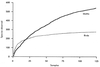
Body size and diversity

Answer 96

Avrage body size, togeter with guild identity allows to infer about abundance.

Question 97

Sampling for biodiversity (issues)

Answer 97

1) Sample size and sampling effort: The number of species and therefore diversity will increase with number of samples. Thus, sample size must be standarized or adjusted for. Ideally, the number of samples should be so to achieve an asympote when plotted with a measure of diversity or eveness.
2) Nonrandomness: Sampling is assumed to be random, but in reality might not be (e.g., environmental heterogeneity, individual behavior).

Question 98

Replication/pseudoreplication

Answer 98

True replicates must be spatially independent.

Question 99

Methodological edge effects

Answer 99

When sampling inefficiency results in concluding one or more species is absent or rare (e.g., sampling methods, sampling time)

Question 100

Measuring abundance: Modular units

Answer 100

Sampling units regarded as different individuals from one larger clonal individual (e.g., fungi, trees, corals). The use of modular units is justified by sub-individuals acting as true individuals ecologically.

Question 101

Measuring abundance: Biomass as an abundance measure

Answer 101

Biomass can be a good surrogate of abundance, and provides information on resource use.
It can also reduce numerical differences between species that vary in their abundances by orders of magnitude.

Question 102

Measuring abundance: Cover area

Answer 102

Cover area can be used as a surrogate of abudnance but is problematic, as organisms can overlap.

Question 103

Measuring abundance: Frequency or incidence

Answer 103

The number of sampling units in which a species occurs. It can be an useful measure for richness.
However, the abundance of widespread species can be underestimated.

Question 104

Comparison of communities: Species abundance distributions

Answer 104

Species abundance patterns can be compared between communities through hypothesis testing (e.g., Kolmogorov-Smirnov test) and slope comparison.

Question 105

Comparison of communities: Rarefaction

Answer 105

Method to measure species richness. A good way of comparing two communities with confidence intervals.
Allows the adjustment of sample size between communties by calculating what richness would be if less samples would have been taken.

Assumes that sampling was truly random.

Note the shape of rarefaction curve is expected to vary depending on the species abundance distribution type.

Question 106

Comparison of communities: Statistical tests

Answer 106

because thr Shannon, Simpson, and other statistics are often normally distributed, they can be compared with t tests and ANOVA.

Question 107

Comparison of communities: Jackknifing

Answer 107

Becaue jackknifing is a nonparametric method, one of its biggest advantages is that it makes no assumption about the underlying distribution of data.

1) diversity (i.e., and index) is estimated for all samples tgether: St
2) diversity is recalculated n times leaving out one sample at a time: St_-i
3) pseudovalues are then calculated for each sample
4) jackknifed estimate is the mean of all pseudovalues
5) SE used to perform t tests

Question 108

Comparison of communities: Bootstrapping

Answer 108

Bootstrapping is a method similar to jackknifing (and considered an improvement). The original data set is repeatedly sampled to produce many combinations of observations and these are used to calculate a standard error.

Question 109

Comparison of communities: Null models

Answer 109

A fairly recent approach to compare a community in question against a series of random draws from a regional pool. Can also be used to test if differences in diversity are an artifact of sampling.

Question 110

Environmental assessment

Answer 110

Environmental assessment evaluates the status of potentially impacted assemblages against a benchmark expectation.

1) Species/abundance distributions: undisturbed assemblaes usually follow a log normal pattern.
2) ABC curves: Placement of individual/biomass curves used to infer on disturbances. W statistic (a measure linking biomass and abundace) can be compared with a sttistical test.
3) Richness: Number of species simply used to infer on disturbance
4) Taxonomic distinctness: Δ⁺ used to infer on ecosystem function.
5) Indices of biotic integrity (IBI’s): integrate a number of metrics; requires extensive background information; not intended for measures of diversity.

Question 111

Turnover

Answer 111

The number of species eliminated and replaced per unit time.
Term is also used sometimes for spatial changes, though β is more appropriate in that situation.

Question 112

Levels of diversity

Answer 112

Inventory diversity:
α diversity: the diversity of a set of samples form one spatial unit
γ diversity: the diversity of a landscape
ε diversity: the diversity of a geographic region

Differentiation diversity:
pattern diversity: variation in diversity between samples from a site
β diversity: the difference in diversity between two spatial units or points in time
𝛿 diversity: change in diversity betwee units of γ (landscapes)

Note: no concensus on how to define a landscape or geographic region.

Question 113

β-diversity and area sampled

Answer 113

Contrary to α, β-diversity decreases as the area sampled increases.

Question 114

Levels of richness

Answer 114

According to Gray (2000):

Scale
point species richness: richness of a sampling unit
sample species richness: richness from a number of samples from one site
large area richness: richness from an area including a variety of habbitats
biogeographic province species richness: richness of a biogeograpic province

Independent of scale
habitat species richness: richness in a habitat
assemblage species richness: richness of an assemblage

Question 115

β-diversity formula

Answer 115

, where S_T is the species richness of the landscape;

• S_j* is the species richness of the assemblage j;
• q_j* is the proportional weight of assemblage j based on its sample size.

Question 116

Measuring β-diversity (trhee main approaches)

Answer 116

1) Difference between 2 areas of α-diversity in respect to γ-diversity (where γ-div is measured as richness); e.g., Whittaker and Lande
2) Similarity/dissimilarity between 2 areas of α-diversity(e.g., Jaccard and Bray-Curtis coefficients)
3) Measuring turnover in terms of the slope in a species-area realtionship

Question 117

Whittaker’s β_{<span>W</span>}

Answer 117

One of the simplest and most effective measures of β-diversity;

β_W = S/(mean α)
or
D_β = S_T/(mean S_j) in Lande;s notation

Values range from 1 to 2; often reported as β - 1 to set the range from 0 to 1

Question 118

Harrison’s modifications of β_W

Answer 118

1) β_H1 = {[(S/mean α) - 1]/(N - 1)} * 100
sets range from 0 - 100

2) β_H2 = {[(S/α_max) - 1]/(N - 1)} * 100
α_max is the maximum within-taxon richness per sample;
Often used to compare turnover of different taxa

Question 119

Other measures of β-diversity

Answer 119

1) Cody’s measure β_C: Focuses on lost vs gaines species

2) Routledge’s measures β_R (takes overlapping distributions into consideration)
β_I (based on information theory)
β_E (the exponential form of β_I)

3) Wilson’s and Smida’s measure β_T (focuses on loss and gain like β_C, but uses average sample richnes like β_W).

Question 120

Wilson and Shmida’s criteria for a good β-diversity measure

Answer 120

1) Number of community changes
2) Additivity
3) Independece from α diversity
4) Independence from excessive sampling

β_W considered the best measure under these criteria

Question 121

Complementarity

Answer 121

Describes the difference between sites in terms of species they support; used for conservation;
Very similar to β-diversity; The more complementary two sites

Question 122

Complementarity measures

Answer 122

Complementarity measres combine three variables: a (species present in both samples), b (species present in sample 1), c (species present in sample 2).

Question 123

Maczewski-Steinhaus measure

Answer 123

Complementarity measure calculated as:
C_MS = 1 - a/(a+b+c)

Question 124

Jaccard’s measure

Answer 124

Complementarity measure calculated as:
C_J = a/(a+b+c)

Question 125

Sorensen’s measure

Answer 125

Complementarity measure calculated as:
C_S = 2a/(2a+2b+2c)

Question 126

Lennon’s measure

Answer 126

Complementarity measure that focuses on differences in composition; calculated as:
β_sim = 1 - [a/a+min(b,c)]
smallest values of b and c are used to avois inflating value

Question 127

C_N = 2jN/(N_a + N_b);
a version of Sorensen that takes abundance into account

Answer 127

A ccomplementarity measure taking abundance into account; calculated as:
C_N = 2jN/(N_a + N_b)

Regarded as the best complementarity measure.

Question 128

Morisita-Horn

Answer 128

Popular complementarity measure that is very sensitive to the abundance of the most abundant species. A way of dealing with that is square transforming the raw data.

Question 129

Estimating the true number of shared species

Answer 129

V is an index to estimate complementarity that focuses on the rare species providing more information than abundant ones.

Question 130

Cluster analysis

Answer 130

A method to compare betwee communties in terms of β-dibversity; Works by constructing dendrograms based on site similarities, where distance is measured. Boostrap values can be added.

Includes dentrograms and ordination.

Question 131

ANOSIM

Answer 131

Analysis of similarities; a one-way nonparametric test using permutations to test a null hypothesis;
Comparisons are made among localities with a number of replicates.

Question 132

Null expectation contrasting

Answer 132

A method to compare communities in terms of β-dibersity.
An observed pattern of β-biodiversity is contrasted against a null expectation.

Question 133

β measure distribution comparison

Question 134

Whittaker’s multiplicative law

Answer 134

Gamma diversity is a product of Alpha and Betta diversity

Question 135

Phytosociology

Answer 135

The science that aims to clasify plant communities into fixed units

Question 136

Niche

Answer 136

An n-dimensional hypervolume composed by environmental and resource characteristics that a species requires to persist (Hutchinson 1959).

Question 137

Assembly rule (Diamond 1975)

Answer 137

A restricted species combination to which competitive ineractions can lead.