Analysis of ecological communities Flashcards
(85 cards)
Biodiversity data reduction
Summarization of how sample units relate to each other, Two types:
- Categorization.
- Creating synthetic variables (e.g., ordination).
Problem with using traditional multivariate tools in community ecology
Data are accompanied by unwanted properties
Questions asked by comunity ecology
What are the species living in an area and why?
What controls diversity?
Ordinal variables
Categorical variables of a ranked nature
Nominal variables
Categorical variables of a qualitative nature with no inherent rank
Dummy variables
Categorical variables with n possible states transformed into binary variables in which 1 or 0 represent presence or absence of something categorical.
Discontinuous variables
Variables with fixed numerical values (e.g., percent)
Continuous variables
Variables with potential infinite numerical values. In practice, seldom true (e.g., set graduations in a measuring device).
Routes for analyzing a species matrix
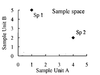
Q route: Relationships among sample units
R: Relationships among species
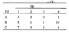
Transposing (matrices)
Flipping a matrix vertically or horizontally.
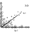
In a normal matrix species are treated as axes;
In a transposed matrix, species are treated as points.
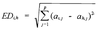
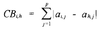
Calculated matrices
Matrices wholes values are calculated from multiplying variables from an original matrix.
Metaobjects
A sample containing objects sich as species, environment, treatment, and species traits.
Columns and rows of a matrix are considered objects.
Each pair of objects can potentially form a different matrix, altough not always conceptually appealing.
Sparse matrix
A matrix containing many zero values.
Relativization
Standarizing a number of variables into a single scale (e.g., number of standard deviations from the mean).
Focal species
A species in a community with special interest (e.g., a rare species interesting for conservation).
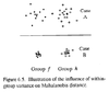
Focal species-habitat relationship
Two ways to examine:
1. Species-centeres approach: predict species performance from habitat variables (e.g., regression)
- Habitat-centered approach: describe variation in habitat variables and evaluate species position within that variation (e.g., ordination).
Sampling (McCune’s definition)
The process of selecting objects of study from a larger number of those objects, where each object is subjected to one or more measurements.
Examples of species abundance measurements
- Cover
- Frequency
- Counts
- Biomass
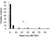
- Basal area
- Importance values (average of >1 sampling measurements)
- Presence/absence
- Size-class data
Types of sampling schemes
- Random
- Stratified random
- Regular (sample units are spaced at regular intervals)
- Arbitrary without bias (haphazard)
- Subjective (e.g., we sampled the most diverse landscapes)
Sources of random numbers
Random number tables, stopwatch, etc.
Types of cover sampling units
- Fixed area: circles, squares, rectanlges
- Point intercept: percent cover is calculated as proportion of hits by points
- Line intercept: percent cover measured as proportion of a line superimposed on a species
- Distance method: Distance from a randomly chosen point to nearest tree (based on the concept that distances can be used to calculate the mean area occupied by an object).
Number of sample units (rule of thumb)
For every imporant controlling factor, 20 additional sample units are needed;
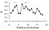
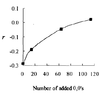
Alternatively, a species accumulation curve can be used to calculate needed number of samples (when a curve flattens out, addiitonal sampling stops being beneficial).
Measures of sample adequacy
Precision: Increases with addiitonal digits.
Accuracy: How close a measurement is from reality
Bias: Any systematic directional error
Measuring accuracy
A sample taken as “the truth” is taken by intensive sampling and resampling an area with dufferent observers and a large number of sampling units.