Venter Factors Flashcards
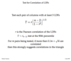
Formulas for Adjusted SSE

Formula for estimating q(w,d), for Cainladder and BF methods
Chainladder: q(w, d+1) = f(d)c(w,d) f(d) is an LDF-1
BF q(w,d)=f(d)h(w) f(d) is proportional to % paid in period d, and h(w) is proportional to an estimate of ultimate losses
Definition of variables in Venter Factors
q(w,d) incremtal paid in row w and age d
c(w,d) cumulative paid
f(d) column parameter
h(w) row parameter
Using a row times column parameter estimate, assume variance is constant for all cells in the triangle. What is the formula for f(d) and h(w)?
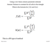
Losses are modeled using f(d)h(w). Assume variance is proportional to expected incremental losses. What is the formula for f(d) and h(w)?
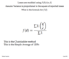
Losses are modeled using f(d)c(w,d). Assume variance is constant for all cells in the triangle. What is the formula for f(d)?
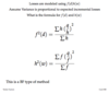
Losses are modeled using f(d)c(w,d). Assume variance is proportional to reported losses. What is the formula for f(d)?

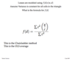
Losses are modeled using f(d)c(w,d). Assume variance is proportional to the square of reported losses. What is the formula for f(d)?
In Venter factors, for an m x m triangle, how many parameters are there when using the:
- Chainladder method
- BF method
- Cape Cod
Chainladder: m-1, one for each column, except the first
BF: 2m-2, same # of column paramters as CL, but also one for each row (except te first)
Cape Cod: m-1, same # of column as parameters as CL
When losses are modeled as f(d)h(w), and we group row and column parameters, how many parameters are there?
of column parameters (don’t count the first column) + # of row parameters (count the first row) -1
How can we test for linearity?
If there is a sequence of negative residuals followed by positive residuals, or vice versa, then the formula for q(w,d) may not be linear
Test for correlation of LDFs
Test for high or low diagonals
Regress the losses against:
- Cumulative loss at prior age
- Dummy variable (0 or 1) for each diagonal
If the diagonal term’s coefficient is twice its standard deviation, we have a high or low diagonal
Model inflation in the BF method
q(w,d) = f(d)h(w)g(w+d)
g(w+d) is the inflation term, and could be:
g(w+d) = (1+j)^(w+d) where, j is the annual inflation rate
Briefly describe six testable implications of Mack’s chain-ladder assumptions.
⇧ Significance of the factor f(d) – the absolute value of f(d) should be at least twice its standard deviation for the factor to be considered significantly di↵erent from zero
⇧ Superiority to alternative emergence patterns – use the sum of squared errors to determine which emergence pattern provides the best fit. Test statistics such as AIC and BIC could be used as well
⇧ Linearity – plot incremental residuals against previous cumulative losses. If the points are randomly scattered around zero, we can assume linearity
⇧ Stability – plot incremental residuals against time (i.e. AY). If the points are randomly scattered around zero, we can assume stability
⇧ Correlation of development factors – calculate the sample correlation coefficients for all pairs of columns in the development factor triangle. Count the number of significant correlations to determine if correlation exists
⇧ Additive CY effects – use regression to determine if any diagonal dummy variables are significant. If so, then an additive CY effect exists and accident years are not independent
Briefly describe three alternatives to the standard chain-ladder emergence pattern.
⇧ Linear with constant – states that the next period’s expected emerged loss is a linear function of the previous cumulative losses PLUS a constant
⇧ Factor times parameter – states that the next period’s expected emerged loss is a lag factor times the expected ultimate loss amount for an AY
⇧ Factor times parameter including a CY effect – states that the next period’s expected emerged loss is a lag factor times the expected ultimate loss amount for an AY times a CY effect factor
Explain why the additive chain-ladder model and the Cape Cod model will always produce the same results.
The Cape Cod model states that the next period’s expected emerged loss is a lag factor f(d) times the expected ultimate loss amount h. Since h does not vary by accident year, this is equivalent to the additive chain-ladder model which states that the next period’s expected emerged loss is a constant g(d) for all accident years. Thus, if we fit the Cape Cod model, we can define g(d) = f(d)h for the additive chain-ladder model. Similarly, if we fit the additive chain-ladder model, we can define f(d)h = g(d) for the Cape Cod model
Briefly describe three methods for reducing the number of parameters needed to fit the Bornhuetter/Ferguson model.
⇧ Assume several accident years in a row have the same mean level
⇧ Fit a trend line through the ultimate loss parameters
⇧ Group AY’s using apparent jumps in loss levels and fit a single h parameter to each group
