Meyers Flashcards
(28 cards)
Diagram of Models Tested

Kolmogorov-Smirnov (KS) Test
D=max |pi-ei|
Reject the null hypothesis (predicted percentiles are normal) if D>136/n.5
LIght Tailed Distributions
Heavy Tailed Distributions
Biased High/Upward
Diagnostics
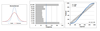
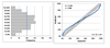
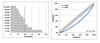
What to look for in the p-p plots
Slope at the right tail & left tail
Shallow Slope indicates the model has a light tail
Steep Slope indicates that model has a heavy tail
Predicted Percentiles are accepted as uniform unless they fail the KS Test at the 5th percentile
Two metrics to test stability in the book of business
- Consistency in net earned premium
- Consistency in the ratio (Net Premium/Direct Premium)
Mack (Incurred)
- Fits a mean & standard deviation to the unpaid losses for each AY
- Overall:
- Light left tail
- Very light right tail
- Fails KS test
- Need to look for a predictive distribution that has fatter tails

Leveled Chain Ladder (Incurred) - LCL
- Add “column” correlation - Treat the value at the last diagonal for the row as a random variable
- u(w,d) = alpha(w) + b(d)
- Has more variance than Mack
- Overall:
- Definite light tails
- Fails KS test
- Improvement over Mack but still forecasts tails that are too light

Correlated Chain Ladder (Incurred) - CCL
- Continue to use “column” correlation
- Add a parameter p to create correlation of losses by AY
- u(w,d) = alpha(w) + b(d) +p(ln(C(w-1,d) - u(w-1,d))
- More variance than Mack
- Overall:
- Very slight light tails on both sides
- Passes KS test
- Meyers concludes this model is good enough

ODP Bootstrap (Paid)
- Overall:
- Very shallow in the left tail
- Looks biased high
- Fails KS test

Mack (Paid)
- Overall:
- Slight shallow right tail
- Very shallow left
- Biased high
- Fails KS test
- Two plausible explainations:
- Insurance loss environment has experienced changes
- Other models can validate

Correlated Chain Ladder (Paid) - CCL
- Continue to use “column” correlation
- Add a parameter p to create correlation of losses by AY
- Overall:
- Biased High
- Fails KS test

1Correlated Incremental Trend (Paid) - CIT
- Add “column” correlation - Treat the value at the last diagonal for the row as a random variable
- Add a parameter p to create correlation of losses by AY
- Add CY trend parameter - t
- Applies to incremental losses
- Overall:
- Biased high
- Fails KS test

2 properties of incremental losses
- Skewed right
- Occasionally has negative values
Tighter variance parameters on which 2 variables for the CIT
- t - CY trend
- sigma (d)
Leveled Incremental Trend (Paid) - LIT
- Add “column” correlation - Treat the value at the last diagonal for the row as a random variable
- Add CY trend parameter - t
- Overall:
- Very light left tail
- Biased high
- Fails KS test

Changing Settlement Rate (Paid) - CSR
- Add “column” correlation - Treat the value at the last diagonal for the row as a random variable
- Add parameter “y” that allows for recognition of a speed up in claim payments
- Overall:
- Fits well
- Removed high bias
- No indication of light tails
- Meyers says this is the best model for paid data

Variance (Meyers)
=E(Process Variance) + Var (Hypothetical Means)
=EVPV + VHM
= Process Risk + Paramter Risk (CF)
Larger component of total risk - Parameter or Process Risk
Parameter Risk
Describe three tests for uniformity for n predicted percentiles

Describe two ways to increase the variability of the predictive distribution produced by the Mack model on incurred losses. For each one, identify a model that accomplishes this goal.

Briefly describe two formulations for the skew normal distribution.
- One formulation produces the skew normal distribution by expressing it as a mixed truncated normal-normal distribution
- Another formulation produces the skew normal distribution by expressing it as a mixed lognormal-normal distribution
Briefly describe why model risk can be thought of as a special type of parameter risk.
Model risk is the risk that we did not select the right model. In a sense, we can think of model risk as a special case of parameter risk because the possible models can be thought of as “known unknowns” similar to the rest of the parameters in the model
