Quant: Common Probability Distributions

Question 1

Probability function/distribution basics =

Answer 1

0 < P(x) < 1

ΣP(x) = 1

Discrete or Continuous (where a single point on a continuous distribution has P(x) = 0

Question 2

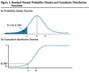
(Cumulative) Distribution function =

Answer 2

Defines the probability that a random variable takes on a value less than or equal to a specific value. F(3) = probability that X is 3 or less

Question 3

Binomial Distribution =

Answer 3

Binomial random variable can be defined as the number of ‘successes’ in a given number of trials (where the outcome can only be success or failure).

Question 4

Bernoulli Random Variable =

Answer 4

Binomial random variable where number of trials is 1

Question 5

Expected value of a binomial random variable =

Answer 5

number of trials times the probability of success (gives the expected number of successes, np

Question 6

Variance of a binomial random variable =

Answer 6

np(1-p)

Question 7

Stock Price Tree/ Binomial Stock Price Model =

Answer 7

Starting stock price, S

P for price movement up and down

Factor for up and down movements

Multiply factors together to get price and probabilities together to get probablity (over multiple periods in the tree)

Question 8

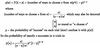
Continuous Uniform Distribution =

Answer 8

Probability between 4 and 8 = 8-4/12-2 = 40%

SUPER EASY

Question 9

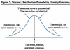
Normal Distribution =

Answer 9

Skewness = 0, Kurtosis = 3.

Linear combination of normally distributed random variables is also normally distributed.

Question 10

Multivariate distribution =

Answer 10

describes the probabilities of group of random variables. Meaningful only if there is a dependent relationship between the variables.

Joint probability table used for two discrete random variables.

Multivariate normal distr for two continuous and normally distributed random variables.

Question 11

Multivariate normal distribution =

Answer 11

is defined by the means and variances of the sets, as well as the pair-wise correlations.

n means,

n variances,

0.5n(n-1) pair wise correlations

Question 12

Confidence Intervals =

Answer 12

Question 13

Standard Normal Distribution/ z-value =

Answer 13

normal distribution that is standardized so mean =0, sd = 1.

Question 14

Shortfall Risk =

Answer 14

probability that a portfolio value or return will fall below a particular (target) value or return over a given time period.

Question 15

Roy’s safety first criterion (like the sharpe ratio) =

Answer 15

optimal portfolio minimizes the chances that returns will fall below a certain threshold value.

MAXIMIZE THE SF RATIO and CHOOSE THE PORTFOLIO WITH THE LARGEST SF RATIO

Question 16

Lognormal distributions =

Answer 16

generated by the function e^x, where x is normally distributed. Note, ln(e^x) = x, so logarithms of lognormally distributed variables are normally distributed.

Question 17

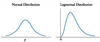
Lognormal distributions and price relatives =

Answer 17

Lognormal distribution has a minimum of 0. This is useful when we model asset prices that can go no lower than 0.

Price relative = end of period price/beginning period price

= 1 + holding period return

Question 18

Continuously compounded rate of return =

Answer 18

EAR = e^Rinfinity -1

to find the annual stated rate that will give the speficied EAR (given continuous compounding), we take the natural log of 1 + rate.

ln(1+EAR) = R_infinity

Question 19

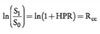
*Continuously compoounded rates of return (additive over multiple periods) =

Answer 19

Question 20

Monte Carlo simulation: What is it?

Answer 20

Simulation technique to generate a distribution of security values, using risk factors that affect these values.

• specify parameters (mean, variance, skewness) and probability distribution of risk/determining factors
• randomly generate values for the specified factors
• ITERATE
• calculate mean security values to use as an estimate of actualy values (could be price/value of a security)

Question 21

Monte Carlo Simulation: Pros/Uses :

Answer 21

• Value complex securities
• Simulate profits/loss from a trading strategy
• Estimate VAR to determine risk in a portfolio
• Simulate variability of assets/liabilities for a pension fund over time
• Value portfolios of assets taht have non-normal returns distributions

Question 22

Monte Carlo Simulation - drawbacks/limitations =

Answer 22

Complex.

Provides answers only as good as the inputs/assumptions

It is a STATISTICAL method, not an ANALYTICAL one.

Question 23

Historical simulation (vs Monte Carlo) =

Answer 23

Uses past data, distribution of risk factors etc.

Shortfall of only considering what happened in that period ie events that happen rarely are unlikely to be considered.

Historical simulation cannot simulate in the ‘what if’ manner that a Monte Carlo can be used for.