Phylogenetic reconstruction Flashcards
Cladistics vs Phenetics
Cladistics: regards combining characters (Apomorphies)
Phenetics: Regards numeric diferences (Distances)
Criterion and method cladistic methods
- Parsimony:
1. Maximum parsimony (MP) - Probabilistic: Likelihood-based:
- Maximum likelihood (ML)
- Bayesian inference (BI)
Parsimony
- Less number of steps
- We expect convergence and reversals
to occur less than synapomorphies - less homoplasy
- # sp = #trees
Advantages and disadvantages Parsimony
Advantages:
Is a simple method - easily understood operation
- Does not depend on an explicit model of evolution
- Gives both trees and associated hypotheses of character evolution
- Should give reliable results if the data is well structured
Disadvantages:
May give misleading results if homoplasy is common or concentrated in particular parts of the tree
Character evolution
History vs model
Observed topology
History: Hypothesis about the evolution of a particular character or a phylogeny
Model: Specifies probability of change between the start and end of each branch
Observed topology: Different scenarios
Assumptions about character evolution
BUT
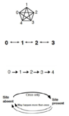
- Unordered (Fitch Parsimony)
- Ordered (Wagner Parsimony)
- Irreversible (Camin-Sokal Parsimony)
- Dollo (Dollo Parsimony): The loss of function is more posible
BUT: there are distances that violate inequality
Compound coding probelms
- Create compound conditions
- each of such condition might legitimately be consider its own character
Multistate coding problems
Phylogenetic information can be lost to the tree search process
Non-additive binary coding problem
Non-additive binary coding makes the absence token (usually 0) correspond to a ‘nonspecified other’ variable: The ‘0’ taken becomes a catch-all for anything that isn’t scored as ‘1’
Search for a Parsimony tree
- Exhaustive search (exact)
- Branch-and-bound search (exact)
- Heuristic search methods (hopefully exact)
Exhaustive search for the Parsimony tree
- Adding 1 more taxon each time
- All posible trees
- Absourd t with more than 10 taxa
Branch and bound search for the Parsimony tree
Looking for short cuts (most likely trees)
- Also t consuming
Heuristic search for the Parsimony tree
- Create a starting tree
- Branch swapping (Randomize the data ser for every search):
- Multiple random search replicates
3. new starting point: change points until: less steps
4. re-start with different order.

Create a staring tree
- • A greedy method
- • Start with 3-taxon tree (Most parsimoniuos)
- • Add taxa one at a time.
- • Keep only the best tree found so far
- • No guarantee of optimality, but may provide good starting point for search
Branch swapping:
- Nearest-Neighbor Interchange (NNI)
- Subtree Pruning and Regrafting (SPR): cutting & pasting different parts of the tree
- Tree Bisection and Reconnection (TBR)
Criterion phenetic
Distance methods
Distance methods
Criterion
Advantages & Disadvantages
Minimum Evolution (ME)
The tree with the shortest sum of the
branch lengths
Advantages:
• Distances can be ‘corrected’ for unseen events.
• Usually faster than character-based methods.
• Can be used for some rate analyses.
-used at the beginning for checking the alignments
Disadvantages:
• Information lost when characters transformed to distances.
• Cannot be used for character analysis.
Examples for distances (ME)
- total number of differences
- p (= uncorrected) distances
- corrected distances following evolutionary models
p- distances = (total # differences)/total # characters
Distance methods tree reconstruction
Neighbor joining

Why Maximum Likelihood
- Multiple substitutions not detectable by parsimony or distance methods
- Observes the likelihood of every character state
in a phylogenetic tree
Parameters of Maximum Likelihood
- Substitution probabilities
- Base composition
Parameter substitution for ML
Transitions more frequent than transversion

Parameter Base composition in ML
- Amount of character states (ACGT)
- varies significantly en very organism
DNA substitutions models
- Jukes-Cantor (JC 1969)
- Kimura 2 parameters (K2P 1980)
- Felstein 1981 (F81)
- Hasegawa, Kishino, Yano (HKY 1985)
- General time reversible models ( GTR 1990)
- Nasty Model
Jukes-Cantor
DNA substitutions models
- Most parsimonious
- Assumes 25% of posibility to each base
- Simple model (1 parameter)
Kimura DNA substitutions model
- @ Transitions
- ß Transvertions
- @ different from ß or else: JC
- 2 parameter
Felstein DNA substitutions model
Unequal base frequencies Π
Substitutions equally likely
2 paremeters
HKY DNA substitutions model
Transversions and transitions with different substitution rates
3 parameters
GTR DNA substitutions model
6 parameter
Takes in to account that all transvertions don´t have the same posibilities
@ is different from ß
All 6 pairs of substitutions have different rates
More to improve a DNA substitutions model
- Proportion of invariant sites
- Gamma distribution
proportion of invariant sites (I)
(improve a model)
sequences that evolve fast may show less divergence than sequences than slower sequences
- Not all nucleotides evolve freely
GTR+I
Gamma distributions (G)
Improve a model
Nucleotides vary differently, some vary more freely than others. Not equally distributed
- Allow more than 2 categories (zero and non-cero rates)
GTR+I+G

How to chose a model
Problem:
The more complex a model, the more computationally expensive.
but:
If a model is too generalizing, the inferred phylogeny can be wrong.
Therefore: Model, that is significant better than
others but does not require more parameters than
necessary.
- Run a model test
Model test
hRLT for nested models
- Likelihood of the different models
- Until there are not significantly differences between the models
Likelihood methods
- Maximum likelihood
- Bayesian inference
- have an explicit probabilistic model
- have statistical basis / support
- search parameters for most likely answer
Bayesian inference (BI) Posterior probability
A priori assumptions
The probability of the event of interest
under certain conditions.
(conditional probability)
Likelihood and Prior probability
Sampling Procedure Markov Chain Monte Carlo
1: Robot is programmed to walk a pre-defined amount of steps (also called
generations), e.g., 2,000,0000
2: Robot evaluates every step in varying length and direction:
- if the step is uphill (higher likelihood): always takes step
- if the step is downhill: 1. robot calculates a height ratio between the steps
2. generates a random number between 0 and 1
3. if number lower than ratio: take the step
if number higher than ratio: it stays at same place
3: Robot evaluates following step…
4: Position (tree topology) of e.g. every 100th step is sampled.

Bootstrap values vs Posterior probabilities
Bootstrap:
Index that best supports the data given, not a true stadistic.
(Split) Posterior Probabilities:
The tree that best supports the data.
When to stop the robot MCMC
- multiple runs (time intensive)
- loooooooong runs (time intensive)
- multiple Markov Chains (robots) simultaneously
(Metropolis Coupled Markov Chain Monte Carlo =
MCMCMC = MC3)
-one chain as usual (cold chain)
-other chains can make larger steps (heated chains)
-chain with the highest probability at every step
becomes automatically cold chain and is sampled.
maximum likelihood vs Bayesian inference
ML
Stadistical knowledge
no priors
Unpredictible running time
Branch support can take ages
Heuristic search: get stuckin local optima
bayes
No stadistical knowledge
Priors
T=linear computational complex
Branch support inmediatly
convergence at burn in
Testing for Robustness of the phylogenetic tree
- Bootstrap
- Jacknife
- Bremer supports (Decay index)
Bootstrap
1) Characters are resampled with replacement
> many (100…1000…10,000)… bootstrap replicate data sets
2) Tree from each bootstrap replicate reconstructed
3) Majority-rule consensus of all trees
> Visualization of agreement in topologies
4) Majority rule consensus indices
= measure of support for those groups
= bootstrap proportions (BPs),
- Tells support, but bot quality of the tree
- Can be wrong if sampled the wrong kind of data
Jacknife
-Jackknifing is very similar to bootstrapping
• differs only in resampling strategy
• proportion of characters (e.g. 50%) is deleted
• Results summarized with a majority-rule consensus tree
• Majority rule indices = Jackknife Probabilities
• Jackknifing and bootstrapping tend to produce:
– broadly similar results
– similar interpretations
- cutting-off characters
Bremer support (Decay index)
- The number of extra steps it takes to collapse a group
- Add aditional steps, to see if the topolofy remains
- The higher the number, higher the support
How to measure Posterior probability?
(conditional probability * Prior probability) / probability of the data given a specific model
How does the robot of MCMC works?
Every step is called a generation
Cloud: Sampling a large amount of potential trees
Program to always go up: down only under certain conditions
Paup index.
- Ci
- Hi
- Ri
Consistency index Ci (Deals with apomorphies)
Ci=( (minimum total SUM of character changes expected)/(actual amount of steps))*100
Also useful to compare trees, to check the amount of homoplasies.
The higher the Ci: the better (how good the data is, and how the characters can be included in the trees)
With Binary characters (0-1): (each character expected to change only one. (parsimony) in the tree)
CI=1 if there is no homoplasy
negatively correlated with the number of species sampled
Homoplasy index Hi: The amount of homoplasies= 1-Ci
0,85-1=-0,15
Retention index
Ri: ((Max steps on the tree - number of state changes in tree)/( Max steps on the tree - number of state changes)
Ri= (Max N. Of steps-Steps observed)/(Max N. Of steps-min. Steps)
defined to be 0 for parsimony uninformative characters
RI=1 if the character fits perfectly
RI=0 if the tree fits the character as poorly as possible