Week 4.7.8: Genetic trait associations Flashcards
(40 cards)
Genetic trait associations
Genetic association studies, genome-wide association studies, missing heritability, genetic disease associations, single gene disorders, polygenic disorders
In previous lectures we have been looking at;
What the human genome looks like
How we sequence genomes
How history shapes genomes
How human genomes differ from the genomes of other species
BUT HOW DO GENOMES INFLUENCE OUR PHENOTYPES? WHAT DO GENOMES DO?
How? What? Why?
A major goal of genomics is to identify which parts of the genome are responsible for which traits. We know that the genome is having a major influence on traits like height – but how is it doing this? How do we get from our DNA too our heart or lungs etc.
Two lines of evidence in genetic trait associations
<!--[if !supportLists]-->
- <!--[endif]-->Genetics
<!--[if !supportLists]-->
- <!--[endif]-->Traits
Two lines of evidence in genetic trait associations
Genetics
Traits
So we have to look at both of those things the genes and the traits –

We know that that baby didn’t come from that couple – because we know looking at the traits, the inheritance of particular traits that the adults have means that it is not likely that baby is from those parents.
We know a lot of the traits we see in this picture are heritable –
Heritability
Of a trait within a population is the proportion of observable differences in a trait between individuals within a population that is due to genetic differences.
Heritability is about the variability of a trait – how much is due to genes and how much is it due to environment, we know that all traits are a mixture of our DNA and environment, thus we know its not just our genes that are responsible for how large your stomach is but if you eat lots of doughnuts you are more likely to have a big stomach – the heritability might be one reason why someone has a big gut but the environment has affect
How do we untangle the difference between genetic and environment effect on traits
One way of doing this is using family studies, and twin studies we know that many human traits have a high heritability. If twins vary in their traits we know that that variability is not due to their genes but due to their environment and so by doing twin studies we can begin to untangle environment and genetic influences.
If we cannot use twins then we can use families instead
We could study plants; we can clone them, growing them in different environments thus controlling genes in that they are clones
However, we cannot do human cloning, even if we did a clone and then had to manipulate their environment it would be very unethical
Facebook experiment – tweeking peoples facebook feed to see if it effected there mood – with loads of backlash
We just can’t do these experiments
But we can work with twin – family studies to try to untangle genetics/environment
We have known about heritability since long before sequencing genome s
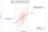
Sir Francis Galton’s (1889) data showing the relationship between offspring height (928 individuals) as a function of mean parent height (205 sets of parents)
Genetics without DNA
From 1850 to 1950 we did genetics without knowing DNA was the hereditary material
We knew about genes since Mendel – even before we knew about DNA
Genetic maps since 1913, Alfred Sturtevant made the first genetic map (a Drosophila chromosome)
Looking at heritability is something we have been able to do for a long time
Two lines of evidence
1.Patterns of heredity – Tracing the inheritance of traits through generations
2.Patterns of DNA variation – DNA sequencing and comparison in multiple individuals
What two type of traits are there?
Two types of traits… Monogenic or polygenic
**What is a monogenic trait? **
Monogenic
A monogeneic trait will often show a clear pattern of Mendelian inheritance, like the peas, either dominant or recessive that segregated in the F2 generation. They tend to be present/absent in phenotype, which are relatively easy to discover the genetic basis for when you can do controlled crosses and generate large families of progeny.
In humans they are a bit harder to work on than in pea plants but still they are fairly easy to work out
However,
Polygenic traits are not…
They are traits that involve many genes, they do not normally show clear Mendelian inheritance as they involve interactions of many genes (many loci interacting)
Polygenic traits are not…
They are traits that involve many genes, they do not normally show clear Mendelian inheritance as they involve interactions of many genes (many loci interacting)
Interact with environment in complex ways, genetic basis can be very hard to discover;
What appraoch do we use to study polygenic traits?
Quantitative trait association studies QTLs
Commonly studied with Genome Wide Association Studies (GWAS)
GWAS is a way of looking at highly polygenic traits
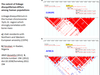
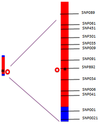
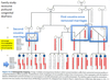
From the textbook chapter 6 figure 6.9
Shows a monogeneic trait and its inheritance in comparison with polygenic traits – we are looking at disorder traits
As we know from Mendelian genetics we have simple inheritance patterns observed on the left – were are polygenic traits are not
We know there are many polygenic traits

Three examples of monogenic traits?
Monogenic
<!--[if !supportLists]-->
· <!--[endif]-->Cystic fibrosis I that is why we have known about its genetic basis for a long time
<!--[if !supportLists]-->
· <!--[endif]-->Sickle cell disease
<!--[if !supportLists]-->
· <!--[endif]-->Phenylketonuria
Three examples of polygenic traits?
Polygenic
<!--[if !supportLists]-->
· <!--[endif]-->Type 2 diabetess
<!--[if !supportLists]-->
· <!--[endif]-->hypertension
<!--[if !supportLists]-->
· <!--[endif]-->rheumatoid arthritis
People are still working on locating loci
Study sampling designs
With humans, we can’t design experiments on genetics as we can with other organisms
We have to make use of what variation and genealogical relationships we can discover existing in human populations
<!--[if !supportLineBreakNewLine]-->
<!--[endif]-->
Which people do I study?
How much of the genome do I study?
Which people do I study?
Two issues when we try to do a study,
Which people do I study?
How much of the genome do I study?
The more humans and the more genome studied the more expensive it will be – but obviously you might be able to learn a lot more looking at more people and their whole genome
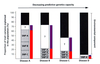
Case control studies
Compare a large group of people showing a trait with a large group of people not showing a trait. For example type 2 D, you get as many people who suffer and as many that don’t then look at all the alleles of those who have type 2 D with those that don’t have – so that if you can find a single allele found in those with type 2 D, you can infer that that allele is something to do with type 2 D
But you have to take account of;
<!--[if !supportLists]-->
· <!--[endif]-->genetic background (everyone from Manchester/Munich)
<!--[if !supportLists]-->
· <!--[endif]-->environmental exposure
<!--[if !supportLists]-->
· <!--[endif]-->same trait but different genetic cause
Works best for discrete traits (Cases/Controls)
Family-based studies
In a family based study you can know the genealogies (you know who the mother was and the father, the granddad and uncle etc.) and you can look at linkage analysis – often the environmental studies will be similar this can help control for environmental effects. Family based studies have been very successful are discovering many Mendelian traits.
<!--[if !supportLists]-->
· <!--[endif]-->More powerful methods
<!--[if !supportLists]-->
· <!--[endif]-->Genetic background and environmental exposures often similar among family members
<!--[if !supportLists]-->
· <!--[endif]-->Problem of numbers – families small
<!--[if !supportLists]-->
· <!--[endif]-->Used to discover basis of many Mendelian traits
<!--[if !supportLists]-->
· <!--[endif]-->May discover rare mutations unique to a family
Might give great results but it might only be particular to that family
Cohort study
You do not just take people at a certain time you study them over a long period of time
This allows for a better understanding of environment, so good for G x E studies
Hard to manage and fund experiments like this is hard in practical
Large population studies
Often used for polygenic quantitative traits that show continuous variation (most polygenic traits do)
Need many sequence data
But this can be hard to get accurate phenotypes – and its expensive to get lots of genotypes and phenotypes
Study design:
How much of the genome do I study?
Candidate gene studies
The candidate gene approach to conducting genetic association studies focuses on associations between genetic variation within pre-specified genes of interest and phenotypes or disease states. This is in contrast to genome-wide association studies (GWAS), which scan the entire genome for common genetic variation.
Focus on particular gene at particular locus, how will you concentrate on a chosen genomic region. Prior knowledge points to that region a previous family based study, a study of a gene function in mice or another organism. (Relatively cheap). Allows you to see if there is variation in that gene. Cheap because you are looking at one thing but it can be very hard to replicate these studies because you might pick up something unique to the sample that is studied
But if you don’t look at candidate genes you do a Genome-wide study
Hypothesis free
Look across the whole genome, little prior knowledge needed
<!--[if !supportLists]-->
Ø <!--[endif]-->using SNP markers or WGS
Expensive – lots of data needed and can be hard to replicate
Complex statistics: big possibility of false positives and negatives, because you are doing MANY statistical tests
Two major types of study
1.Linkage analysis (Linkage mapping)
2.Genome wide association studies (Linkage disequilibrium mapping)
These two approaches take eliminates from types of studies and how many people and genome do you study
Linkage analysis (Linkage mapping)
Brings together the two lines of evidence
·heredity patterns of traits
·genome sequence
You need to know pedigree of every individual
You can start off as a genome-wide search, but then you need to do sequential studies needed to gradually narrow down the genomic region for a trait’s locus. Can begin with a candidate region of the genome
The main aim of linkage analysis is that you want to identify genetic markers that segregate with a trait of interest
Two lines of evidence
·Patterns of segregation of a trait in families
·Patterns of segregation of genetic markers in same families
Segregation happens because:
·Chromosomes segregate in meiosis (between mum and dad)
· Recombination segregates loci within chromosomes
We have known about this for a very long time,
Genetic distance

Genetic distance between two loci is measured by the recombination fraction
If 1% of progeny from a cross are recombinant, then they are 1 centimorgan apart (1 cM)
i.e. if a trait co-occurs with a marker in 99% of the progeny of a cross, the marker is likely to be 1cM from the trait locus
Genetic distance and physical distance are somewhat different, in terms of bases, because recombination is more frequent at parts on the chromosome – they look further apart than they actually are
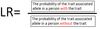
LOD Scores
Measure of linkage between loci, Log10 of the likelihood ratios between the observed linkage and the null hypothesis of no linkage at all
·LOD score above 3 may suggest significant linkage
·LOD score of less than -2 may suggest no linkage
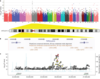
Genome wide association studies (GWAS) (Linkage disequilibrium mapping)
Linkage disequilibrium mapping
Do not need to know pedigrees
Hypothesis free
Look across the whole genome
<!--[if !supportLists]-->
· <!--[endif]--> using SNP markers or WGS
How often does each locus have a variant that co-occurs with the disease?
How often does each locus have a variant that co-occurs with the disease?
Little prior knowledge needed
Expensive – lots of data needed
Can be hard to replicate different cohorts of samples can give different results
Complex statistics: false positives and negatives
Bus Analogy
3.2 billion seats, something goes wrong when seat number 116572 is occupied by a male
But all we know is which buses have gone wrong, and who was on each bus
How do we associate “male in seat 116572” with the problem?
This is very difficult what we have to do is look across all the buses and find occupants of the seats of all the different buses and find the seat that is always the same in the individual buses with the problem – mathematically that is a difficult problem – look for something very small in very large data set
What helps us is linkage disequilibrium
our 3.2 billion loci are not randomly assorting in our genomes we don’t have 3.2 billion chromosomes – we only have 23 chromosomes
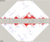
Although recombination is happening within those chromosomes its not enough that the 3.2 billion are segregation randomly in EVERY generation – because it does not happen all that frequently along the chromosome we find that there are lots of block in the structure of the variation within the human genomes so lots of loci are linked when we look at human populations. That is linkage disequilibrium if something was in equilibrium, it would mean that everything is randomly assorted as if we have 3.2 billion chromosomes.
As we get further away on both sides they are less linked in many ways conceptually they are similar to linkage mapping (but in linkage mapping we are just looking at one family or one pedigree where we are tracing a lineage and tracing recombination events)
Linkage disequilibrium we are just looking at populations we are not looking at linkage pedigree we are just observing these patterns as a phenomena that is arising – but we are exploitation the fact that linkage disequilibrium occurs so we can associate blocks with one another and this means that when we are looking for an allele associated with a trait we can look for a block of loci that are linked –