Topic 3

Question 1

Define Free energy qualitatively. How does free energy relate to whether a reaction proceeds or not?

Answer 1

• Useful work that can be obtained from the system
• A reaction proceeds when system has the ability to perform work or when change in free energy, ΔA is negative.

Question 2

Define Free energy thermodynamically. What kind of ensemble is used?

Answer 2

• ΔA = ΔE-TΔS
• A = Helmholtz free energy
• E = Internal energy
• T = Temperature
• S = Entropy
• Generally done under NPT ensemble, however here canonical (NVT) ensemble described for simplicity.

Question 3

What type of systems cannot be simulated usind MD? Give examples of biological systems we can simulate and how the free energy there is related to the processes.

Answer 3

• In MD, classical forcefields can’t be used for reactions involving bond breaking/making.
• Protein folding and ligand binding are ideal applications for this
• ΔE and ΔS define whether a protein fold is favourable enough to form and how strongly a ligand binds to a protein.

Question 4

Discuss changes in free enrgy, binding and structure as well as solvent reorganisation in a ligand binding system

Answer 4

• Binding of the ligand will cause a change in enthalpy/internal energy as a result of intermolecular interactions (e.g. electrostatic interaction associated with vdW)
• Loss of conformational freedom in binding site causes a decease in entropy, that counterbalances an increase due to water around free ligand having more freedom.
• The total free energy is a net effect of all these different changes

Question 5

Experimentally we can find the free energy of a system using ΔA = -RTlnK_bind where K_bind is the ratio of the time a ligand is bound compared to unbound. Why does this approach not work for simulation and what is an alternative approach?

Answer 5

• To sufficiently sample a system in both states, and directly calculate the free energy would involve simulation times that are too unrealistic.
• Instead relate the free energy to a microscopic description of the system through statistical mechanics
• A = -k_bTlnQ_NVT­, (Q_NVT is the canonical partition function)

Question 6

• Canonical partition function, Q_NVT tells us the total number of … a system can access through summing all possible state’s … and …

Answer 6

• Canonical partition function, Q_NVT tells us the total number of microstates a system can access through summing all possible states positions and momenta

Question 7

What are some problems with using a partition function approach to calculate free energy directly? What is an alternative approach

Answer 7

• Sampling entire phase space and integrating Q_NVT directly is impractical
• Alternatively, could take an ensemble average, and give A in terms of potential energy, U. (A ∝ e^-U(r))
• However low energy samples would contribute very little average (?) and high energy samples take a long time to reach.
• This leads us to not being able to calculate A directly.

Question 8

Alternatively, we can use the free energy difference to calculate ΔA between an initial state (0) and final state (1). Briefly, give an example of an initial and final state system as well as how we arrive at being able to use this as our method.

Answer 8

• An initial state may be an unbound ligand or unfolded protein, with a corresponding bound/folded final state.
• We can therefore solve ΔA = -k_bTlnQ_1­/Q₀

Question 9

• Q_NVT is a function of the …, which depends on the sum of … (…) and … (…) energy as a function of … and …
• … can be solved analytically, leaving … as an excess which can be calculated in a simulation at each step giving overall …

Answer 9

• Q_NVT is a function of the Hamiltonian, which depends on the sum of kinetic (K) and potential (U) energy as a function of position and momenta.
• K can be solved analytically, leaving U as an excess which can be calculated in a simulation at each step giving overall ΔU.

Question 10

What is an ensemble average and how is it applied to our calculation of ΔA?

Answer 10

• Ensemble average is an average over all microstates generated from a simulation in a given state. In our case, P, is the property in our snapshot* probability distribution (related to Q)
• We can now calculate ΔA from a single simulation in the ensemble corresponding to state 0

Question 11

How is our method of calculating ΔA as a function of ΔU implemented?

Answer 11

• Carry out simulation of state 0, calculating PE at each step (U₀)
• At each step also, take configuration (snapshot of trajectory) and apply PE function corresponding to state 1 to calculate U₁, resulting in ΔU.
• This is known as thermodynamic perturbation theory

Question 12

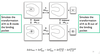
How might we compute the difference in hydration free energy between two ions?

Answer 12

• Define forcefield parameters for Lithium in a box of water, as well as for rubidium in water.
• Water terms are identical, Li and Rb will have different LJ/coulombic terms
• Run MD simulation of system in state 0 (Li_(aq)⁺), calculating U₀ via PE eqn and terms defined in FF.
• Simultaneously, take same configuration and calculate PE of system in state 1 (Rb_(aq)⁺), U₁
• Same coordinates, only difference is parameters used to calculate U₁ and therefore ΔU at that step.
• At end of simulation take average of ΔU and use to find ΔA.

Question 13

How might we compute binding free energy difference between ligand B and ligand A?

Answer 13

• Physical changes in binding are difficult to simulate accurately in MD simulations (in addition to the longer length of time it takes to wait for event to occur)
• Instead we can simulate the non-physical transfer of A to B inside and outside the pocket.
• Parameters associated with A (state 0) will differ from those of B (state 1)
• At each step we can calculate the energy of A in/out of the pocket and that of B in/out the pocket to find ΔU, then average ΔU over the simulation.

Question 14

What is the problem ignored so far in free energy calculation using thermodynamic perturbation theory with no windows? relate your answer to the free energy of the system

Answer 14

• If state 0 and 1 are very different (state 0 has a low probability of being in state 1) then ΔU is large
• In the case of Li/Rb this would occur due to unfavourable interactions of Rb overlapping the water molecules closer to Li, causing a high energy LJP term
• A large ΔU results in the large exponential term becoming negligibly small, giving low weight in ensemble average
• This causes ΔA to converge slowly, meaning our errors in our finite simulation will be large.

Question 15

What is the solution to our free energy perturbation theory problem?

Answer 15

• Break down calculation into windows where there is good overlap between states and ΔU is small.
• This is done through a coupling parameter, λ, which gradually increases from 0 to 1 through multiple simulations (equation), then sum the free energy changes outputed
• There is an increase in cost for these additional simulations
• In Li/Rb case first window would be change from Li to 10% Rb etc

Question 16

What is an example of the solution to energy perturbation theory?

Answer 16

• The free energy change in mutating AA glycine to Alanine might be an important system to study for active site manipulation.
• As λ increases from 0 to 1 we switch off interaction of glycine and turn on interaction of alanine.
• This shows the power of simulations as this is impossible experimentally
• A technical issue with this is that as we switch LJ interaction changes as charges are switched on/off gradually, causing atoms to shift to unfavourable locations.

Question 17

• Describe a simple alchemical transformation of zero-sum ethane, describing initial and final states

Answer 17

• Dual-topology hybrid molecule used to describe alchemical transformation
• One methyl group vanishes at one end of the molecule and one appears at the other
• Initial state, λ = 0 (black); final state, λ = 1 (brown)

Question 18

• Describe the results of the free energy change associated with the alchemical transformation of zero-sum ethane. What conditions have this simulation been performed under and what is the consequence of that?

Answer 18

• Simulation has been done in the absence of a soft core potential
• This results in end point catastrophes as well as high energy fluctuations giving overall poor convergence

Question 19

Why don’t the forward and backward reactions give the same result?

Answer 19

• Interactions of vanishing/appearing atoms with surrounding atoms/molecules (not each other as simulation incoming/outgoing moieties don’t ‘see’ each other’)
• These interactions will differ depending on which way the reaction proceed

Question 20

• What is a soft-core potential?

Answer 20

• An interatomic potential that differs from a LJP used to describe the interatomic forces and therefore potential of a system.
• It does not account for interactions between vanishing and appearing chemical moieties, preventing high energy fluctuations in doing so
• Interactions at short range are effectively dampened compared to a LJ potential.
• Atoms approaching each other very closely (at end-point catastrophise – high/low λ values) will give a much lower energy than a standard LJP