Key notes final

Question 1

What do computer simulations do and what do they allows?

Answer 1

Allow the study of properties of a many body system by creating a mathematical model (e.g a molecular mechanics forcefield) to describe the system behaviour which can be run to sample configurational space of that system (main families are MS and MC)

Question 2

Why bother using comupter simulations?

Answer 2

• Gain better understanding of the system at a molecular level which allows better design of experiments and help interpret data.
• Predict properties/behaviour from molecular structure.
• Simulate unrealistic experiments that explore extreme conditions or toy models (e.g turn off charges to investigate hydrophobic driven reactions)

Question 3

What is an MD simulation and what does it allow us to do?

Answer 3

• Enable us to simulate the time evolution of a system of particles.
• Can extract thermodynamic and kinetic information through simulation of particles at a position at the beginning and end of many steps.
• Trajectories are generated through classical dynamics (ignore electronic effects) by solving newtons equations of motion.

Question 4

How are newtonian principles employed in MD simulations?

Answer 4

• The force acting on an atom i due to all other particles in a system is linked to the potential experienced by atom I and its position
• Using newtons second law (F=ma) we can also find the particles acceleration

Question 6

Why can MD trajectories not be solved analytically? What must be done instead

Answer 6

• Cannot be solved analytically for a many-body system as force acting on each particle depends on the position of all other particles at that moment in time.
• Instead F=ma is solved numerically using small time steps Δt (~fs) where the force is calculated at the end of each of these time steps then following on to the next one.
• Most commonly done with the Verlet algorithm

Question 7

What defines the transferability of a force-field?

Answer 7

• The ability to re-use fore-field parameters across a range of different functional groups.
• More parameters may be accurate for a specific system but transfer poorly to another.
• Forcefields have been paramaterised to reproduce properties of proteins, lipids e.g CHARMM, AMBER. Same functional form but differing parameters (different torsion angle for amino acids)

Question 8

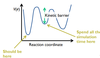
Ergodicity is not always true in practice, why is this?

Answer 8

• A barrier that is too high can cause system to be kinetically trapped in a certain region of phase space, leaving the global minimum unexplored.
• If one is doing a grid-based lattice simulation getting stuck in local minima when starting on certain set of lattice coordinates can be a problem.

Question 10

What are periodic boundary conditions (PBC)?

Answer 10

Convenient way of representing bulk solution without having to simulate every molecule where molecules are placed in a simulation cell replicated in all three directions via minimum image convention

Question 11

What is the time scale problem? What is a chemcial example that suffers from this?

Answer 11

• Larger than that of length scale, avoiding getting stuck in local minima can use up most simulation time without sampling desired configurational space.
• Can occur if waiting for a rare event to occur, but instead getting stuck behind a kinetic barrier.
• No way to know if this has occurred as the PES is not available prior to the simulation.

Question 12

What are edge effects and how are they overcome?

Answer 12

• Many small boxes have many atoms, some of which are close to edge.
• Results will be influenced by particles interacting with the edge of the system.
• Edge effects are overcome by having molecules that pass through the cell walls appear on the other side.

Question 13

Assuming MM suffices over QM, what is the length scale problem?

Answer 13

• System must be a manageable number of particles; however systems are growing larger (millions of atoms).
• One must choose the system carefully to get desired output.

Question 14

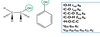
Briefly discuss and compare three different force-fields, using the alcohol octanol as an example.

Answer 14

• All-atom: An all atom/atomistic force-field treats each atom explicitly. At every step, the simulation must input all bonding/non-bonding interactions in a system. In long molecules like octanol, this can lead to many dihedral angles needing to be specified for all differing ~-OH chains. Very precise however, computationally costly.
• United-atom: cheaper way to describe the system that saves computational time, but still expensive. It does this by grouping less chemically involved hydrogen atoms into CH­₂ groups. Good for lipid descriptions
• Coarse graining: 4-5 heavy atoms with their H’s are grouped into a single interaction site, saving large amount of computational effort. Octanol is split into a polar (hydrophilic) and non-polar (hydrophobic) half. Lose a degree of chemical detail as cannot capture hydrogen bonding explicitly. However partial charges assigned to these blocks to describe electrostatic and non-bonding interactions.

Question 16

What are three ways in which coarse graining allow simualtion on larger systems for longer timescales?

Answer 16

• Decrease in total number of particles N
• Larger time step
• Smoother energy landscape

Question 17

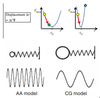
How does larger time-step ‘speed up’ a coarse grain simulation?

Answer 17

• A ​time step for integration needs to be smaller than the highest frequency motion in a system.
• The verlet algorithm can be used to move an atom through calculation of the force, with respect to all other atoms, to apply in one timestep, which should be constant.
• A time step may be suitable for bond stretch of a low frequency (left), resulting in it being closer to its equilibrium value. However, the same force acting on a higher frequency motion (right) results in a high energy final position, leading to assumption of force being constant over our chosen timestep to be invalid.
• Timesteps should be 10x smaller than highest frequency motion, which are generally bond stretches of light hydrogen atoms.
• By removing bonds involving them, a larger time step can be used, as particles of higher mass oscillate slower. Each time step now propagates us further forward in time.

Question 18

How does a decrease in total number of particles N ‘speed up’ a coarse grain simulation?

Answer 18

• A decrease in total number of particles reduces the number of force calculations required at each step.
• Resulting in less computational time needed to move the system forward one-time step, as less forces and energies must be calculated each step.

Question 20

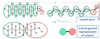
How does a smoother energy landscape ‘speed up’ coarse graining?

Answer 20

• Rugged energy landscape of an atomistic model has many local minima.
• Averaging that occurs through coarse-graining results in a smoother energy landscape with less local trapping/friction and faster dynamics.
• Beads can slide over each other much easier

Question 21

Why must we develop new interaction potentials for coarse grained systems?

Answer 21

• Coarse-grained particles do not interact in the same way that atoms do.
• New coarse-grained potentials must be developed that are unique to each system.
• Parameterising is a large challenge as takes a lot of time to predict the correct output.

Question 22

What are two methods of generating course-grained interaction potentials?

Answer 22

• Use an analytical functional form with associated parameters; like atomistic interaction potentials but with CG beads
• Numerically fitting data from atomistic simulations using tabulated potentials (list of r’s between atoms with corresponding F’s/E’s – useful for complex systems where don’t have analytical function)

Question 23

What is mapping, and why is it essential for developing a CGP? (PPQ)

Answer 23

• The first stage in developing a CG interaction potential (CGP) is to define mapping of the atomistic system in to a CG one.
• Essential for new molecules and there are many ways to assign atomistic structure depending on what interactions are expected to be the focus.

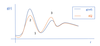
Question 24

What is an RDF?

Answer 24

• A radial distribution function g(r) shows the probability of finding a particle at distance r from a reference particle.
• At small distances there is a low probability of finding another atom due to coulombic repulsion (LJP?)
• Shells form around the reference particle as other bands of particles appear, with depletion zones between them.

Question 25

What are 2 general rules of mapping?

Answer 25

• Each bead will inherit the mass/charge of its constituents
• Must maintain the overall shape of the molecule (otherwise may not replicate the correct self-assembled structure)

Question 26

Outline how you would produce a CG trajectory from an atomistic simulation using a bottom up approach

Answer 26

• First, run a reference atomistic simulation to use as our benchmark (however does not necessarily equal experimental/ab initio PES)
• Extract effective CG potentials using a trajectory of a system (a series of snapshots over time).
• Each snapshot in the atomistic simulation will have positions for all atoms at each timestep which will be used to find their corresponding Force/Energy.
• A CG pseudo trajectory can be attained by grouping atoms in to beads using the beads centre of mass based on an atomistic average.

Question 27

• How does our improved guess for the intermolecular CG potential [V^CG_i+1(r)] change when g_i(r) = g_ref(r)? – 1 on graph

Answer 27

k_BTln…= 0, no change to interaction potential needed as CG simulation produces same pairwise structure as atomistic

Question 28

• How does our improved guess for the intermolecular CG potential [VCGi+1(r)] change when g_i(r) ref(r)? – 2 on graph

Answer 28

• k_BT… is -ve
• probability of finding particle (correlation between CG beads) at that r underestimated.
• Equation will lower pairwise CG energy at that r, making interaction more favourable

Question 29

• How does our improved guess for the intermolecular CG potential [VCGi+1(r)] change when g_i(r) ref(r)? – 3 on graph

Answer 29

• k_BTln… is +ve
• probability of finding particle (correlation between CG beads) at that r overestimated.
• Equation raises pairwise CG energy at that r, making interaction more appropriately favourable (less than before).

Question 31

How does an RDF used as a target reference functions help form non-bonded potentials from the trajectory of a system?

Answer 31

• Goal is to form a CGP that reproduces the RDF obtained from atomistic simulations.
• The CG RDF, g(i) is linked to the trajectory of our system CG trajectory,
• Which in turn is linked to an atomistic RDF, g(ref), derived from an atomistic trajectory.

Question 32

How is V_PMF used in Iterative Boltzmann Inversion iteratively?

Answer 32

• V_PMF =k_BTln[g_ref(r)] instead is used as a starting guess for V_CG (intermolecular CG potential)
• V_i+1^CG(r) = V_i^CG(r) + k_BTln[g_i(r) / g_ref(r)] is our improved guess after each iteration
• g_ref(r) is our target probability distribution from atomistic simulation
• g_i(r) is the probability distribution from a CG simulation using the i^th potential
• Difference between the two moves us closer of further to result

Question 36

• Why does it take so long to produce a CG potential through IBI that is like an atomistic trajectory?

Answer 36

• Must iteratively calculate each pairwise interaction in your system using the IBI method until a full CG tabulated potential that is like the original atomistic trajectory is gained.
• However once this is done, CG allows us to reach much higher simulation times.

Question 37

• What is a problem with the IBI discussed in lectures as well as an example of this being solved?

Answer 37

• It takes only a singular atomistic simulation into account as a reference that will be under certain set conditions. This is a problem if one wanted to study phase transitions, which are dependent temperature changes.
• Moore et al (2016) developed a CGP constructed using many different atomistic simulations at varying temperatures to account for this, known as multi-state IBI.

Question 38

• What is force matching and how does it differ to Iterative Boltzmann inversion?

Answer 38

• IBI tried to match the structure of an atomistic simulation where the RDF is used to reach our target data.
• Force matching aims to match forces on the CG interaction sites with the forces at the atomistic level.

Question 39

• What are some advantages of both bottom-up and top-down approaches?

Answer 39

• Bottom-up: capable of capturing fine detail of interaction as CG interactions are extracted from reference atomistic simulations
• Top-down: provide potentials that are more easily transferable and applicable to experimental data.

Question 40

• What is an example of a top-down approach?

Answer 40

• The MARTINI force field, a CG potential fitted to reproduce experimental target data, using few parameters and standard interaction potentials to maximise transferability.
• A choice of building blocks calibrated against experimental oil/water partition coefficients are available to build a system

Question 41

• What is a disadvantage of the MARTINI force-field?

Answer 41

• No systematic way for developing potentials and introducing new molecules unavailable in building blocks.

Question 42

• What are some disadvantages of CG models?

Answer 42

• A model can be too biased, and very untransferable to another system
• A model may only be parameterised for a specific class of molecules, showing a lack of compatibility
• Model may be too coarse to capture desired behaviour

Question 43

What type of systems cannot be simulated usind MD? Give examples of biological systems we can simulate and how the free energy there is related to the processes.

Answer 43

• In MD, classical forcefields can’t be used for reactions involving bond breaking/making.
• Protein folding and ligand binding are ideal applications for this
• ΔE and ΔS define whether a protein fold is favourable enough to form and how strongly a ligand binds to a protein.

Question 44

Discuss changes in free enrgy, binding and structure as well as solvent reorganisation in a ligand binding system

Answer 44

• Binding of the ligand will cause a change in enthalpy/internal energy as a result of intermolecular interactions (e.g. electrostatic interaction associated with vdW)
• Loss of conformational freedom in binding site causes a decease in entropy, that counterbalances an increase due to water around free ligand having more freedom.
• The total free energy is a net effect of all these different changes

Question 45

Experimentally we can find the free energy of a system using ΔA = -RTlnK_bind where K_bind is the ratio of the time a ligand is bound compared to unbound. Why does this approach not work for simulation and what is an alternative approach?

Answer 45

• To sufficiently sample a system in both states, and directly calculate the free energy would involve simulation times that are too unrealistic.
• Instead relate the free energy to a microscopic description of the system through statistical mechanics
• A = -k_bTlnQ_NVT­, (Q_NVT is the canonical partition function)

Question 46

What are some problems with using a partition function approach to calculate free energy directly? What is an alternative approach

Answer 46

• Sampling entire phase space and integrating Q_NVT directly is impractical
• Alternatively, could take an ensemble average, and give A in terms of potential energy, U. (A ∝ e^-U(r))
• However low energy samples would contribute very little average (?) and high energy samples take a long time to reach.
• This leads us to not being able to calculate A directly.

Question 47

How is our method of calculating ΔA as a function of ΔU implemented?

Answer 47

• Carry out simulation of state 0, calculating PE at each step (U₀)
• At each step also, take configuration (snapshot of trajectory) and apply PE function corresponding to state 1 to calculate U₁, resulting in ΔU.
• This is known as thermodynamic perturbation theory

Question 48

How might we compute the difference in hydration free energy between two ions?

Answer 48

• Define forcefield parameters for Lithium in a box of water, as well as for rubidium in water.
• Water terms are identical, Li and Rb will have different LJ/coulombic terms
• Run MD simulation of system in state 0 (Li_(aq)⁺), calculating U₀ via PE eqn and terms defined in FF.
• Simultaneously, take same configuration and calculate PE of system in state 1 (Rb_(aq)⁺), U₁
• Same coordinates, only difference is parameters used to calculate U₁ and therefore ΔU at that step.
• At end of simulation take average of ΔU and use to find ΔA.

Question 49

What is the problem ignored so far in free energy calculation using thermodynamic perturbation theory with no windows? relate your answer to the free energy of the system

Answer 49

• If state 0 and 1 are very different (state 0 has a low probability of being in state 1) then ΔU is large
• In the case of Li/Rb this would occur due to unfavourable interactions of Rb overlapping the water molecules closer to Li, causing a high energy LJP term
• A large ΔU results in the large exponential term becoming negligibly small, giving low weight in ensemble average
• This causes ΔA to converge slowly, meaning our errors in our finite simulation will be large.

Question 50

What is the solution to our free energy perturbation theory problem?

Answer 50

• Break down calculation into windows where there is good overlap between states and ΔU is small.
• This is done through a coupling parameter, λ, which gradually increases from 0 to 1 through multiple simulations (equation), then sum the free energy changes outputed
• There is an increase in cost for these additional simulations
• In Li/Rb case first window would be change from Li to 10% Rb etc

Question 51

• Q_NVT is a function of the …, which depends on the sum of … (…) and … (…) energy as a function of … and …
• … can be solved analytically, leaving … as an excess which can be calculated in a simulation at each step giving overall …

Answer 51

• Q_NVT is a function of the Hamiltonian, which depends on the sum of kinetic (K) and potential (U) energy as a function of position and momenta.
• K can be solved analytically, leaving U as an excess which can be calculated in a simulation at each step giving overall ΔU.

Question 52

What is an example of the solution to energy perturbation theory?

Answer 52

• The free energy change in mutating AA glycine to Alanine might be an important system to study for active site manipulation.
• As λ increases from 0 to 1 we switch off interaction of glycine and turn on interaction of alanine.
• This shows the power of simulations as this is impossible experimentally
• A technical issue with this is that as we switch LJ interaction changes as charges are switched on/off gradually, causing atoms to shift to unfavourable locations.

Question 55

What is biased sampling?

Answer 55

• Where a biasing potential is used that can be used to force the system to explore unfavourable configurations, leading to enhanced sampling of phase space
• This means we are more likely to overcome kinetic barriers that trap us in local minima of our PES for our entire simulation time

Question 56

What is a key condition of biased sampling?

Answer 56

Need to know something about pathways as a starting point as this is what we are defining

Question 57

What are reaction coordinates and briefly give two examples? (also known as collective variables and order parameters)

Answer 57

• Characterise a process in terms of a small set of properties of a system that are a function of atomic coordinates.
• Also known as collective variables and order parameters
• Distance/separation, r
• Dihedral angle

Question 58

• Give an example of how distance can be used as a reaction coordinate

Answer 58

• Potential mean force (PMF), which is the free energy along a chosen reaction coordinate, can be simulated using the distance between an Na⁺-Cl^- ion pair in electrolyte solution.

Question 59

• Give an example of how radius of gyration (R_gyr) can be used as a reaction coordinate. What must be assumed?

Answer 59

• R_gyr gives an indication of the expansion/contraction of a globular structure through the average of the distance each atom is from the centre of mass. More expanded = higher R_gyr
• The transformation of a β hairpin peptide to unfolded random coil state’s free energy landscape can be investigated
• Choosing appropriate set of reaction coordinates is difficult so must guess generally

Question 60

Give an advantages and disadvantages of using multiple reaction coordinates

Answer 60

Pros

• A combination of variables allows important structures across high energy barriers to be sampled, giving a larger indication of the greater free energy landscape.
• If our single reaction coordinate output poorly maps experimental results, a second coordinate can be introduced to form a 2D plot that may give a different minimum energy pathway to before.

Cons

• However, in combination, outputs of these reaction coordinates can lead to many different structures which must all be considered
• Certain structures may even be resritcted via specific choice of a given set of coordinates
• Large computational cost

Question 61

• Give an example of how root mean squared distance (RMSD) can be used as a reaction coordinate
• WHat must one be careful of?

Answer 61

• RMSD is the difference between atomic positions at time t and the starting positions of the simulation, t₀.
• Can be averaged over all atoms of interest, e.g. carbons in a protein backbone chain
• Similarly, with R_gyr, must be careful with choice of reaction coordinate to pair with as may not be unique function of r^N.

Question 62

• Free energy is a … function so the free energy change is independent of the …. This means we can create unrealistic … if …/… are not of importance to us.

Answer 62

• Free energy is a state function, so the free energy change is independent of the path. This means we can create unrealistic pathways if mechanism/kinetics are not of importance to us.

Question 63

What factors control the overlap sampling between adjacent simulations and how fine grained our sampling of our free energy profile is in umbrella sampling?

Answer 63

• Force constant
  
  • Too low: biasing insufficient to explore high energy regions (wide harmonic)
  • Too high: insufficient overlap between windows (narrow (harmonic)
• Frequency of window spacing
• Choosing these values is largely trial and error

Question 64

What is the WHAM algorithm?

Answer 64

• The weighted histogram analysis method is used to stitch simulations together iteratively in umbrella sampling.
• Unbiased distribution solved with arbitrary values of free energy associated with that potential.
• Values fed back in to each other until FEP is converged and best estimate for unbiased distribution is obtained.

Question 65

What is metadynamics and how does it differ from umbrella sampling?

Answer 65

• In umbrealla sampling we forced the system to explore unfavroubale regions of phase space with a biasing potential, which restrained us in places difficult to sample, but penalised when too high/unfavourable
• Metadynamics instead adds biasing potentials to penalise the system from visiting already sampled regions (i.e low energy phase space), forcing it to move to less favourable positions

Question 66

• Where umbrella sampling used … as its … potentials, instead, metadynamics uses … … , which are added to the potential as the simulation proceeds. Metdynamics is …, meaning we don’t need to estimate the underlying … … … (and biasing potential) in advance with metadynamics as we did in … …. However, we do still need a reaction coordinate.

Answer 66

• Where umbrella sampling used harmonics as its biasing potentials, instead, metadynamics uses Gaussian functions, which are added to the potential as the simulation proceeds. Metdynamics is adaptive, meaning we don’t need to estimate the underlying energy landscape (and biasing potential) in advance with metadynamics as we did in umbrella sampling. However, we do still need a reaction coordinate.

Question 67

• Outline the basic principles of umbrella sampling

Answer 67

• System is restrained (through tethering to a spring) to a small region along the reaction coordinate ξ using a biasing potential.
• If the system deviates too far from this small region, an energy penalty restores the region.
• This is repeated at different target values of ξ. The system is forced to explore small unfavourable regions along a certain channel until full reaction coordinate is explored.
• All simulations are stitched together to produce an unweighted underlying free energy profile.

Question 68

How does metadynamics allow sampling of the full reaction coordinate?

Answer 68

• Start at some configuration, depositing gaussians as we sample
• Eventually will be pushed out into a new local minimum
• We can tweak how often these depositions occur as well as the height and width of them.

Question 69

• Metadyanimcs can be … … … but is useful for getting a quick scan of the … …

Answer 69

• Metadyanimcs can be slow to converge but is useful for getting a quick scan of the energy landscape.

Question 71

Describe the Monte Carlo (MC) method and how does it contrast to MD method?

Answer 71

• MC simulations are an alternative method to sampling accessible microstates of the ensemble, generally used for smaller systems. Uses orthogonal techniques
• MD used Netwon EOM to predict positions of atoms at a future time, taking a time average to find property of interest
• MC generates configurations through random numbers that are unconnected in a timescale, using an ensemble average to investigate a property

Question 72

How is MC implemented?

Answer 72

• Move a random particle in a predefined way (e.g along z-axis), with an acceptable dr
• Calculate U of new configuration. If lower than original, new configuration is accepted and replaces old.
• A trajectory-esque profile forms as we move to lower energy configurations.

Question 73

How does the size of ΔU affect the acceptance ratio?

Answer 73

• U_new­ > U_old : Boltzmann factor of energy difference closer to 1. More likely to be greater than random # from 0 -> 1. High probability uphill likely favourable) move accepted and added to growing ensemble of microstates
• U_new >> U_old (e.g a steric clash): less random #’s likely to be lower than Boltzmann factor of ΔU. Low probability large uphill move accepted.
• Low energy states are general preferred in this algorithm

Question 74

What are some advantages of MC? Give examples and comparisons to MD

Answer 74

• MC does not need to follow realistic pathways, so can explore conformations more rapidly. E.g. a protein folding event in MD would have to physically fold realistically – slow process. MC could randomly rotate an important dihedral to quickly generate states on interest
• MC doesn’t require calculation of force, whereas in MD, the differentiation of the potential (=F), using Verlet, can be very costly. In MC this isn’t required, allowing for more unphysical models to be used.

Question 75

What is a disadvantage of MC?

Answer 75

• Sampling efficiency depends strongly on move set choice. Poor choice may limit transfer to other unknown configurations, preventing access to all regions of phase space (poor sampling).
• For example, the choice of certain dihedral to sample be our change to sample around, but it may in fact prevent certain configurations from being explored due to unknown factors.

Question 76

What is an example of an MD-MC combined simulation? Why must they be used toghether? How? What is the advantage or combining both methods?

Answer 76

• A mixed lipid-membrane of chains differing by 4C’s in their tail.
• MD would be too slow to see lipid diffusion
• MC would converge too slowly with a system this complex
• Instead a trail MC move follows each MD step, removing/adding 4C atoms, evaluating E of exchange to see if favourable
• Sampling more efficient as removed dependency on starting configuration, which can trap system in very low energy configurations surrounded by high.

Question 77

Why is it difficult to enhance sampling with a biasing potential?

Answer 77

• The timescale problem in MD makes in difficult to overcome kinetic barriers in our simulation time.
• To enhance the sampling of this phase space we could use a biasing potential to explore unfavourable configuration but requires knowledge of important factor in pathways.

Question 78

What is Replica Exchange Molecular dynamics (REMD)?

Answer 78

• REMD is an alternative method of overcoming (or removing) kinetic barriers, allowing more rapid sampling of phase space.
• Can either change the potential via alteration of the forcefield to change the curve we are sampling (H-REMD)
• Or change the temperature we sample at (T-REMD).

Question 79

What is the problem with simply changing the temperature we sample at?

Answer 79

• The conditions in which we have chosen to investigate are now different, which can complicate the system of interest, if an event is temperature dependent (e.g a phase change)

Question 80

• How can we change the temperature more suitably in T-REMD?

Answer 80

• Use Temperature Replica Exchange Molecular Dynamics
• Run an MD simulation of different replicas of the system at different temperatures in parallel (parallel tempering = replicas are generated through MC instead)
• Our temperature of interest is the lowest.
• Exchange configurations between replicas using MC (in both methods)
• Continue simulation
• Repeat step 2 until converged.

Question 81

What is the process of the T-REMD method?

Answer 81

• As in MC, interested in the free energy difference between states.
• If E lower make swap
• If not random number decided if accepted or not
• If accepted take high temperature coordinate simulation and exchange with low temperature configuration
• Overtime, periodic exchanges between replicas allow inaccessible regions of phase space, at high T initially, are now accessible (takes a long time for this to occur though)

N.B. These are not unfavourable regions, they are merely blocked by high E barriers from being sampled -may be lower energy minima

Question 82

What is a disadvantage of T-REMD?

Answer 82

• States are not connected in time
• Can’t use to calculated time dependent properties (e.g diffusion coefficients) as timescale used is unrealistic

Question 83

Discuss the practical considerations that need to be taken in a T-REMD experiment in terms of computational power.

Answer 83

• Many more processors are required to run many replicas in parallel. This along with the size of the system will be tied to the computational resource available.

Question 84

What is the general principle in Metropolis MC?

Answer 84

• The probability of a transition from configuration 1 to 2 is a function of the change in ΔU between those states.
• The probability of a configuration can be written in terms of the Boltzmann distribution where the ideal partition function is a normalizing factor

Question 85

What if the energy of the new configuration is greater than or equal to (≥) original configuration?

Answer 85

• Boltzmann probability is compared to a random number between 0 and 1
• If #_rand < p(new), confuguration accepted, allowing an increase in energy
• If #rand > p(new), new configuration rejected and have another copy of original microstate set

Question 86

What is the process of H-REMD? Give a biological example of where this may be useful

Answer 86

• Temperature across simulations is constant
• Instead a soft-core potential is used to across replicas, where Lennard Jones potential gradually softened meaning that atoms can sit on top of one another while still remaining in certain conformations
• Useful in ligand binding, where certain bound conformations can be locked in deep minima.
• H-REMD allows ligand to rotate in pocket and explore different orientations while still being bound.
• These can then be swapped in to a correct LJP, giving an indicator to the transitions in between them

Question 87

Discuss the practical considerations that need to be taken in a T-REMD experiment in terms of temperatures used.

Answer 87

• Set of temperatures used such that largest temperature will enable rapid exploration of phase space.
• Finding this temperature can be difficult when don’t know the PES
• Spacing between temperatures must also be optimised to minimise convergence time

Question 88

Discuss the practical considerations that need to be taken in a T-REMD experiment in terms of acceptance probability.

Answer 88

• Must run a test to see if exchange if often/probable enough to reach convergence.
• Otherwise, may just switch back and forth between two states of similar energy.

Question 89

Discuss the practical considerations that need to be taken in a T-REMD experiment in terms of the chemistry of the system.

Answer 89

• If one is simulating a system involving a phase change due to increased temperature, this will result in a high energy change (e.g a protein unfolding.
• Must have a lot of replicas around phase transition of configurations that suddenly differ largely.