Section A: Meyers, Taylor & Marshall Flashcards
Taylor: What are the results of Taylor’s Theorems?
Theorems 3.2 and 3.3 are similar to 3.1 about the ODP Mack model and mean:
- Forecasts from the ODP Mack and ODP Cross-Classified models are identical and the same as those from the chain ladder method despite the different formulations.
- We can get forecasts for the ODP Cross-Classified model without considering the model directly and working as if the model was an ODP Mack model.
Marshall: Preparing the Claims Portfolio:
Considerations for Splitting into Valuation Classes
- Preferable to split the claims portfolio into valuation classes the same as the split used to derive the central estimates
- This allows analyzed sources of uncertainty to be aligned with the central estimate analysis.
- If the valuation of the central estimate is at a granular level, it may make sense to do the quantitative analysis on aggregated valuation classes (which are more credible) and allocate results down.
Taylor: Tweedie Sub-Family
Expected Value & Variance

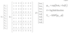
Taylor: ODP Cross-Classified Model GLM Representation (for a 4 x 4 triangle)
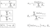
Taylor: The expected value and variance of an EDF:
E[Y] = ?
Var[Y] = ?
E[Y] = µ = b’(𝜃)
Var[Y] = a(ɸ)b’‘(𝜃)
Taylor: The Exponential Dispersion Family (EDF) is the family of distributions with probability density function (pdf) π(y;𝜃,ɸ)of the form:
ln(π(y;𝜃,ɸ)) = ?
ln(π(y;𝜃,ɸ)) = [y𝜃 - b(𝜃)] / a(ɸ) + c(y,ɸ)
y = value of observation Y
𝜃 = location parameter called canonical parameter
ɸ = dispersion parameter called scale parameter
b(•) = cumulant function which determines shape of distribution
ec(y,ɸ) = normalizing factor producing unit total mass for the distribution
Meyers: Bayesian Loss Models
Correlated Incremental Trend (CIT) Formulas
µw,d= ⍺w+ βd + 𝜏(w + d - 1)
Zw,d ~ lognormal(µw,d, σd)
IncLoss1,dsim ~ normal(Z1,d, 𝝳)
IncLossw,dsim ~ normal(Xw,d + ⍴(IncLossw-1,dsim - Zw-1,d)e𝜏,𝝳) for w>1
- LIT model is the same, but sets ⍴ = 0
Marshall: Calibrating balance scorecard scores to CoVs
Example Scale and Comments
Meyers: Non-Bayesian Models
Briefly describe how the ODP Bootstrap model on paid data performed in the Meyers paper?
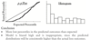
- Histogram shows more low percentiles than expected
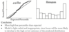
- p-p plot shows a slanted “U” curve
- K-S test fails at the 5% level for all the lines combined
Conclusion
The ODP Bootstrap model is biased high
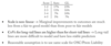
Meyers: Describe three tests for uniformity for n predicted percentiles.
- Histogram - if percentiles are uniformly distributed, the bars should be of similar height
-
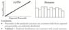
p-p Plot - sort the predicted percentiles into increasing order, then plot the expected percentiles on x-axis and sorted predicted on y axis.
- sorted predicted percentiles should follow the expected percentiles along the 45 degree line
- {ei} = 100*{1/(n+1), 2/(n+1),….,n/(n+1)}
-
K-S Test - reject hypothesis of uniformity if D>D* at 5% level of significance
- D = Max | pi - fi |
- Critical Value = 136 / √n
- fi = 100 * {1/n, 2/n,….,n/n} where n is the # of percentiles
- On a p-p plot, these critical value appear as 45 degree bands that run parallel to the line y=x. We reject the hypothesis of uniformity if the p-p plot lies outside the bands.
Marshall: What is the goal of External Benchmarking?
Goal - compare the reasonableness of CoVs and risk margins to those from external sources.
Should NOT be relied on instead of analysis, but may be useful when there is little information available for analysis; especially for independent risk.
Marshall: External Systemic Risk
Latent Claim Risk
Latent Claim Risk
- Negligible for most valuation line classes but material for some Workers Compensation and liability classes
- Low probability risk with very high potential severity (e.g. Asbestos)
- If the risk exposure is significant enough to be included in the central estimate valuation or capital adequacy modeling, then it should be examined more closely for setting risk margins
- Discuss with underwriters to identify sources of latent claim risk
Marshall: Preparing the Claims Portfolio:
Allocation of Valuation Classes to Claim Groups
- If different groups of claims within a valuation class have materially different uncertainty, they should be treated separately in the risk margin analysis
- e.g Splitting the Home portfolio between CAT and non-CAT claims, splitting non-CAT between liability and non-liability
- Balance the benefit gained and the practicality/cost
Marshall: External Systemic Risk
Claim Management Process Change Risk
Claim Management Process Change Risk
- Typically impacts all valuation classes with different levels of materiality
- Discuss current and future process changes with claims management
- Consider impact on reporting/payment patterns, closing and reopening rates, and case estimation
- Could do sensitivity testing of key valuation assumptions to help assess CoV for this category
- Likely to be more relevant for OSC than premium liabilities
Taylor: The standardized Pearson residuals are defined as follows:
RiP = ?
RiP = (Yi - Yhati) / σhat<strong>i</strong>
Check residual plots against each variable:
- Standardized Pearson residuals should be random about zero (unbiased) and have uniform dispersion (homoscedasticity)
Marshall: Independent Risk Assessment for Oustanding Claim Liabilities
Goal - a model is used to “fit away” past systemic episodes in order to analyze the residual volatility and get the CoVs for independent risk.
Methods Used
- Mack Method
- Bootstrapping
- Stochastic Chain Ladder
- GLM Techniques
- Bayesian Techniques
Marshall: External Systemic Risk
Event Risk
Event Risk
- Catastrophes have most material impact on Property
- Include in OSC liability if there are outstanding events
- Information to help quantify risk for premium liabilities:
- past experience from event risk - could create frequency/severity model and then adjust past experience for changes in portfolio/inflation/…
- CAT models which produce a range of possible outcomes for modelled events on an insurer’s book
- Reinsurance intermediaries
Marshall: External Sytemic Risk CoV Consolidation Formula
CoV2<em>external</em> = ∑CoVi2
- Formula should be similar to internal as some external risks are correlation (within the same class or between PL and CL)
Taylor: ODP Mack Model GLM Representation

Marshall: Summary of Risk Margin Analysis Framework
Marshall: Describe the internal benchmarking that should occur for the following source of risk:
Independent Risk
Portfolio Size: larger portfolios have lower CoVs due to lower volatility from random effects
Length of Claim Runoff: Longer tailed lines have higher CoVs due to more time for random effects to have an impact
Implications:
Long-tailed portfolios - premium liability CoV should be higher than claim liability CoV
Short-tailed portfolios - premium liability CoV should be lower than claim liability CoV
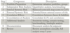
Marshall: What are the sources of Systemic Risk?
Internal Systemic Risk
Risks internal to the liability valuation process
→ Reflects the extent to which the actuarial valuation approach is an imperfect representation of complex, real-life process
External Systemic Risk
Risks external to the actuarial modeling process
→ Even if the model represent the current conditions well, future systemic trends may cause future experience to differ from current expectations
Taylor: What do you need to do to specify a GLM?
The selection of a GLM consists of the following:
- Selection of a cumulant function, controlling the model’s error distribution
- Selection of an index p, controlling the relationship between the models means and variance
- Selection of the covariates xiT
- the variables that explain ui
- Selection of link function, controlling the relationship between the mean ui and the associated covariates
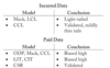
Meyers: Interpreting Diagnostics
Light-Tail Model