Portfolio Management Flashcards
Arbitrage Pricing Theory (APT) - value of Ri
- the intercept is the expected return of asset i given that all the other factors take on a value of 0

APT assumptions
- A factor model describes asset returns
- There are many assets, so investors can form well-diversified portfolios that eliminate asset-specific risk, not factor risk
- No arbitrage opportunities exist among well-diversified portfolios
APT E(Rp) given that the 3 assumptions of the model hold

Pure factor portfolio (or factor portfolio)
A portfolio with a sensitivity of 1 to factor j and a sensitivity of 0 to all other factors
Carhart four-factor model notation (extension of the Fama and French model)
- RMRF = the return on a value-weighted equity index in excess of the one-month T-bill rate
- SMB = small minus big, a size (market capitalization) factor; SMB is the average return on three small-cap portfolios minus the average return on three large-cap portfolios
- HML = high minus low, the average return on two high book-to-market portfolios minus the average return on two low book-to-market portfolios
- WML = winners minus losers, a momentum factor; WML is the return on a portfolio of the past year’s winners minus the return on a portfolio of the past year’s losers
Carhart four-factor model / Rp - Rf

Carhart four-factor model / E(Rp)

Types of multifactor models
- Macroeconomic
- Fundamental
- Statistical:
- Factor analysis - best explain historical return covariances;
- Components models - best explain historical variances
bik for the fundamental factor model

Active return formula
- Asset allocation or sensitivity factor
- Security selection factor

Information ratio (IR)
- = Active return / Active risk
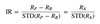
Active risk (also called Tracking error (TE)) - formula
- s(Rp - RB)
- s(RA)
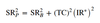
Active risk squared (active risk is also called tracking error or tracking risk) - formula
s2 (Rp - RB)
Active risk squared decomposition
- Active risk squared = Active factor risk + Active specific risk
- Active factor risk and active specific risk refer to variances rather than standard deviation
- Active factor risk
- Active specific risk or security selection risk
- The contribution to active risk squared resulting from the portfolio’s different-from-benchmark exposures relative to factors specified in the risk model
- The contribution to active risk squared resulting from the portfolio’s active weights on individual assets as those weights interact with assets’ residual risk
Portfolio alpha
Active specific risk formula
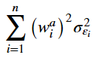
Active specific risk notation
- wai is the ith asset’s active weight in the portfolio (that is, the difference between the asset’s weight in the portfolio and its weight in the benchmark)
- σ2εi is the residual risk of the ith asset (the variance of the ith asset’s returns left unexplained by the factors)
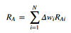
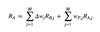
Value added formula
- RAi = Ri - RB
- Ri = return to asset i
- RB = return on the benchmark portfolio
- Δwi = wP,i – wB,i
Value added as the sum of the active asset allocation decisions and the weighted sum of the value added from security selection, RA,j = RP,j – RB,j, within each asset class

The first (parenthetical) term above is the value added from the asset allocation decision. The second term is the value added from security selection within the stock and bond portfolios. The active weights in the first term refer to differences from the policy portfolio
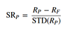
Sharpe ratio
Sharpe ratio for leveraged portfolio
- STD of the risk-free cash (1 - wp) is 0
- RC = wPRP + (1 – wP)RF

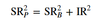
(Sharpe ratio)2p
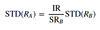
The level of active risk that leads to the optimal result for unconstrained portfolios
The level of active risk that leads to the optimal result for constrained portfolios
Maximum value of the constrained portfolio’s squared Sharpe ratio
The total risk of the actively managed portfolio is the sum of the benchmark return variance and active return variance

Mean–variance-optimal active security weights for uncorrelated active returns

Grinold rule
- Si represents a set of standardized forecasts of expected returns across securities (also called scores)
- σi are multipliers (separate values for individual securities)
- μi are the forecasted active returns

Mean–variance optimal active weights using the Grinold rule

Information coefficient (IC) - formula
/
IC is the ex ante risk-weighted correlation

E(RA)* - optimal expected active return

IR* - information ratio of the unconstrained optimal portfolio

E(RA) of the full fundamental law

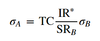
Transfer coefficient (TC) - definition
The TC is the cross-sectional correlation between the forecasted active security returns and the actual active weights, adjusted for risk
Transfer coefficient (TC) - formula

Information ratio (IR) of the full fundamental law

The expected value added conditional on the realized information coefficient, ICR

Realized active return RA considering noise - formula

The IR for a constrained portfolio generally decreases
With the aggressiveness of the strategy
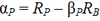
Active return does not equal alpha
RA = RP – RB, while αP = RP – βP × RB
Unconstrained Portfolio
An investment style that does not require a fund or portfolio manager to adhere to a specific benchmark. Unconstrained investing allows managers to pursue returns across many asset classes and sectors
μi - the security’s expected active return
μi = E(RAi)
Active weights

RAi

RAi as the residual return in a single-factor statistical model

Aggressiveness of the active weights impact on the information ratio
- The information ratio is unaffected by the aggressiveness of the active weights (deviations from benchmark weights) because both the active return and the active risk increase proportionally
- The aggressiveness will only decrease the IR of a constrained portfolio

Portfolio variance

Portfolio variance for a portfolio with equal weights 1/N
- σ2 overlined = average variance
- Cov overlined = average covariance

Capital allocation line (CAL)

Capital market line (CML)

Capital market line (CML) versus capital allocation line (CAL)
The capital market line (CML) is the capital allocation line formed when the risky asset is a market return rather than a single-asset return
Portfolio variance for a portfolio of two assets

CAL and the Sharpe ratio
The Sharpe ratio is the slope of the CAL
Markowitz efficient frontier
- The graph of the set of portfolios offering the maximum expected return for their level of risk (standard deviation of return)
*
Market model (single-index model) - return, variance and covariance

- Factor portfolio
- Tracking portfolio
- A portfolio with a factor beta equal to one for one factor and zero for all other factors. Factor portfolios have higher active factor risk (which refers to the deviation of a portfolio’s factor betas from those of the benchmark)
- A portfolio with factor betas equal to those of the benchmark
Macroeconomic models
- The intercept ai is the expected return to stock i
- All other factors have an expected value of 0 and represent a surprise
Ex post IR
- = tb0 / (number of observations)1/2
- = t-value for the intercept / square root of the number of observations
Value added from α
- α = IR * ω
- VA = α - (λ - ω2)
- ω = residual risk
- λ = risk aversion
- α = expected value of the active return
*tested in 2015
Information ratio from α
- IR = α / ω
- ω = residual risk
- α = expected value of the active return
Information ratio additivity
- IRnew2 = IRa2 + IRb2
- The IR of the new stocks can simply be added to the IR of those already managed
Portfolio constraint
- Time horizon
- Liquidity
- Tax concerns
- Legal and regulatory factors
- Unique circumstances
The alpha and information ratio of a portfolio consisting of only cash and the benchmark
Both the alpha and the information ratio are 0
IC using the number of successful decision
- IC = 2(Nc / N) - 1
- Nc = number of correct decisions
- N = total number of decisions
Sharpe ratio and cash
The Sharpe ratio is unaffected by the addition of cash or leverage in a portfolio and would thus not be appropriate to evaluate a portfolio in which an allocation to cash was a key part of the investment decision process
The Fundamental Law of Active Management separates the expected value added, or portfolio return relative to the benchmark return, into the basic elements of the strategy
- Skill (information coefficient)
- Portfolio construction (transfer coefficient)
- Breadth (number of independent decisions per year)
- Aggressiveness (benchmark tracking risk)
