Module 4 – Single Variable Linear Regression Flashcards

1
Q

Given the regression equation, Selling Price = 13,490.45 + 255.36(HouseSize) Selling Price = 13,490.45 + 255.36(HouseSize), what do you expect the selling price of a 900 square foot home to be?

A

The expected selling price of a 900 square foot home is B15+B16*900=$243,314.45. You must link directly to the values in order to obtain the correct answer.

2
Q

Do you feel confident of the prediction you just made for a 900 square foot house, given the data available?

  • Yes
  • No
A

Yes

900 lies well within the range of our historical housing data, so we can feel relatively comfortable with this prediction.

No

See correct answer for explanation.

3
Q

Given the regression equation, Selling Price = 13,490.45 + 255.36(HouseSize), where House Size is measured in square feet, what happens to the average selling price (in dollars) for houses whose size are increased by 500 square feet?

  • Average selling price would remain the same
  • Average selling price would increase by approximately $255
  • Average selling price would increase by approximately $13,490
  • Average selling price would increase by approximately $12,750
  • Average selling price would increase by approximately $127,500
A

Average selling price would remain the same

The average selling price would remain the same when house size increases only if the coefficient for House Size were equal to zero, that is, if the regression line’s slope were equal to zero, then the regression line would be flat. In that case, there would be no expected change in selling price for any increase or decrease in the house size. The slope of our regression line, about 255 dollars/square foot, describes the expected change in price when house size increases by one square foot. If house size increases by 500 square feet, how much will the average price increase?

Average selling price would increase by approximately $255

The slope of our regression line, about 255 dollars/square foot, describes the expected change in price when house size increases by one square foot. If house size increases by 500 square feet, how much will the average price increase?

Average selling price would increase by approximately $13,490

The y-intercept of our regression equation is approximately $13,490. The slope of our regression line, about 255 dollars/square foot, describes the expected change in price when house size increases by one square foot. If house size increases by 500 square feet, how much will the average price increase?

Average selling price would increase by approximately $12,750

The slope of our regression line, about 255 dollars/square foot, describes the expected change in price when house size increases by one square foot. If house size increases by 500 square feet, how much will the average price increase?

Average selling price would increase by approximately $127,500

The slope of our regression line, about 255 dollars/square foot, describes the expected change in price when house size increases by one square foot. If the square footage increased by a factor of 500, the expected price must also increase by a factor of 500. Therefore, the average increase in price as square footage increases by 500 square feet is 500($255)=$127,500.

4
Q

Which of the following p-values would indicate that we can be 95% confident that there is a significant linear relationship between two variables? Select all that apply.

  • 0.0025
  • 0.0100
  • 0.9500
  • 0.9750
A

0.0025

We reach a specified level of confidence when our p-value is less than 1-confidence level. Since the p-value, 0.0025, is less than 1-0.95=0.05, we can be 95% confident that there is a significant linear relationship. Note that another option is also correct.

0.0100

We reach a specified level of confidence when our p-value is less than 1-confidence level. Since the p-value, 0.0100, is less than 1-0.95=0.05, we can be 95% confident that there is a significant linear relationship. Note that another option is also correct.

0.9500

We reach a specified level of confidence when our p-value is less than 1-confidence level. The p-value, 0.9500, is greater than 1-0.95=0.05 so we cannot be confident that there is a significant linear relationship.

0.9750

We reach a specified level of confidence when our p-value is less than 1-confidence level. The p-value, 0.9750, is greater than 1-0.95=0.05 so we cannot be confident that there is a significant linear relationship.

5
Q

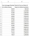
The spreadsheet below contains a partial view of data about U.S. corn acreage planted (in millions of acres) and the amount of corn (in millions of bushels) in storage from the previous year at the beginning of the year for each year from 1976 to 2013.

We wish to use the data to predict the number of acres of corn that will be planted, based on the beginning corn stock in storage. Which variable is the independent variable?

  • Corn Acreage Planted (in million acres)
  • Stock of Corn at Start of Year (in million bushels)
A

Stock of Corn at Start of Year (in million bushels)

“Stock of Corn at Start of Year” is the independent variable, and “Corn Acreage Planted” is the dependent variable. The beginning stock of corn at the start of the year will be used to predict the number of acres of corn that are planted.

6
Q

Given the regression equation, Selling Price=$13,490.45+$255.36(House Size), what happens to the average selling price (in dollars) for houses whose size are decreased by 1000 square feet?

  • Average selling price would decrease by approximately $268,490
  • Average selling price would increase by approximately $268,490
  • Average selling price would decrease by approximately $255,000
  • Average selling price would increase by approximately $255,000
A

Average selling price would decrease by approximately $268,490

The slope of our regression line, about 255 dollars/square foot, describes the expected change in price when house size increases by one square foot. If house size decreases by 1,000 square feet, how much will the average price decrease?

Average selling price would increase by approximately $268,490

The slope of our regression line, about 255 dollars/square foot, describes the expected change in price when house size increases by one square foot. If house size decreases by 1,000 square feet, how much will the average price decrease?

Average selling price would decrease by approximately $255,000

The slope of our regression line, about 255 dollars/square foot, describes the expected change in price when house size increases by one square foot. If the square footage decreased by a factor of 1,000, the expected price must also decrease by a factor of 1,000. Therefore, the average decrease in price as square footage decreases by 1,000 square feet is -1,000($255) =-$255,000.

Average selling price would increase by approximately $255,000

The slope of our regression line, about 255 dollars/square foot, describes the expected change in price when house size increases by one square foot. If house size decreases by 1,000 square feet, average selling price will also decrease.

7
Q

Postive, Negative, or Zero slope?

AS X INCREASES, Y DOES NOT CHANGE.

A

Zero

8
Q

Postive, Negative, or Zero slope?

AS X INCREASES, Y DECREASES.

A

Negative

9
Q

Postive, Negative, or Zero slope?

AS X INCREASES, Y INCREASES.

A

Positive

10
Q

Create a Dummy variable or not?

DIRECTION (NORTH, SOUTH, EAST, AND WEST)

A

Dummy

Variables that can be sorted or grouped into categories must be transformed into dummy variables. Note that numerical values sometimes represent a qualitative/categorical variable, requiring the use of a dummy variable.

11
Q

Create a Dummy variable or not?

TEMPERATURE (IN DEGREES CELSIUS)

A

No

Variables that can be counted or measured and that are naturally represented as numbers do not need to be represented as a dummy variable.

12
Q

Create a Dummy variable or not?

VOLUME (IN CUBIC METERS)

A

Not

Variables that can be counted or measured and that are naturally represented as numbers do not need to be represented as a dummy variable.

13
Q

Create a Dummy variable or not?

COUNTRY TELEPHONE CODE

A

Yes

Variables that can be sorted or grouped into categories must be transformed into dummy variables. Note that numerical values sometimes represent a qualitative/categorical variable, requiring the use of a dummy variable.

14
Q

A p-value to test the significance of a linear relationship between two variables was calculated to be 0.0210. What can we conclude? Select all that apply

  • We can be 90% confident that there is a significant linear relationship between the two variables.
  • We can be 95% confident that there is a significant linear relationship between the two variables.
  • We can be 98% confident that there is a significant linear relationship between the two variables.
  • We can be 99% confident that there is a significant linear relationship between the two variables.
A

We can be 90% confident that there is a significant linear relationship between the two variables.

Since the p-value, 0.0210, is less than 1-0.90=0.10, we can be 90% confident that there is a significant linear relationship between the two variables. Note another option is also correct.

We can be 95% confident that there is a significant linear relationship between the two variables.

Since the p-value, 0.0210, is less than 1-0.95=0.05, we can be 95% confident that there is a significant linear relationship between the two variables. Note another option is also correct.

We can be 98% confident that there is a significant linear relationship between the two variables.

Since the p-value, 0.0210, is greater than 1-0.98=0.02, we cannot be 98% confident that there is a significant linear relationship between the two variables.

We can be 99% confident that there is a significant linear relationship between the two variables.

Since the p-value, 0.0210, is greater than 1-0.99=0.01, we cannot be 99% confident that there is a significant linear relationship between the two variables.

15
Q

Given the regression equation, Selling Price = 13,490.45 + 255.36(HouseSize), what do you expect the selling price of a 425 square foot home to be?

A

The expected selling price of a 425 square foot home is B15+B16*425=$122,018.45. You must link directly to the values in order to obtain the correct answer.

16
Q

Do you feel confident of the prediction you just made for a 425 square foot house, given the data available?

  • Yes
  • No
A

Yes

See correct answer for explanation.

No

425 square feet lies just outside the range of our historical housing data. Remember that there is greater uncertainty as we forecast outside of the historical range of the data, so we probably should not feel very comfortable with this prediction.

17
Q

Given the regression equation, Selling Price = 13,490.45 + 255.36 (HouseSize), which of the following values represents the value of Selling Price at which the regression line intersects the vertical axis?

  • Selling Price
  • $13,490.45
  • $255.36
  • House Size
A

Selling Price

Selling Price is the dependent variable in this equation.

$13,490.45

13,490.45 is the y-intercept, the value at which the regression line intersects the y-axis. This happens when House Size = 0, giving the equation: Selling Price = 13,490.45+255.36*0 = 13,490.45

$255.36

255.36 dollars/square foot is the line’s slope, which is equal to the average change in selling price as house size increases by one square foot.

House Size

House Size is the independent variable in this equation.

18
Q

When analyzing a residual plot, which of the following indicates that a linear model is a good fit?

  • Patterns or curves in the residuals
  • Increasing size of the residuals as values increase along the x-axis
  • Decreasing size of the residuals as values increase along the x-axis
  • Random spread of residuals around the y-axis
  • Random spread of residuals around the x-axis
A

Patterns or curves in the residuals

Patterns or curves in the residual plot indicate that the linear model is not a good fit. It is possible that a nonlinear relationship exists between the independent and dependent variable. What characteristics of a residual plot might indicate that a linear model is a good fit?

Increasing size of the residuals as values increase along the x-axis

The size of the residuals should not increase as values increase along the x-axis; this is a sign of heteroskedasticity. What characteristics of a residual plot might indicate that a linear model is a good fit

Decreasing size of the residuals as values increase along the x-axis

The size of the residuals should not decrease as values increase along the x-axis; this is a sign of heteroskedasticity. What characteristics of a residual plot might indicate that a linear model is a good fit?

Random spread of residuals around the y-axis

The y-axis of a residual plot represents the size of the residuals; this is not the axis that we examine. What characteristics of a residual plot might indicate that a linear model is a good fit?

Random spread of residuals around the x-axis

A linear model is a good fit if the residuals are spread randomly above and below the x-axis.

19
Q

The spreadsheet below contains a partial view of data about U.S. corn acreage planted (in millions of acres) and the amount of corn (in millions of bushels) in storage from the previous year at the beginning of the year for each year from 1976 to 2013.

If you want to include the variables’ labels in the regression output, which cells should you select as the input range for the independent variable?

  • Input Y Range, B1:B39
  • Input Y Range, B2:B39
  • Input X Range, B1:B39
  • Input X Range, B2:B39
A

Input Y Range, B1:B39

The Input Y Range is used to enter the cell reference for the dependent variable, not the independent variable.

Input Y Range, B2:B39

The Input Y Range is used to enter the cell reference for the dependent variable, not the independent variable.

Input X Range, B1:B39

The Input X Range is used to enter the cell reference for the independent variable. The cell reference, B1:B39, correctly includes the column label.

Input X Range, B2:B39

The Input X Range is used to enter the cell reference for the independent variable. The cell reference should include cell B1, since we include the column labels to ensure that our charts are appropriately labeled.

20
Q

Given the regression equation, Selling Price = 13,490.45 + 255.36 (HouseSize), which of the following values represents the value of House Size at which the regression line intersects the horizontal axis?

    • 52.83 square feet
  • 13,490.45 square feet
  • 255.36 square feet
  • The answer cannot be determined without further information.
A

- 52.83 square feet

The regression line intersects the horizontal axis when Selling Price = $0, that is, when House Size = -52.83 square feet. 13,490.45+ 255.36*(-52.83)=$0.00 (actually, -52.82914, which rounds to -52.83).

13,490.45 square feet

$13,490.45 is the y-intercept, the value at which the regression line intersects the y-axis. This happens when House Size = 0 square feet, giving the equation: Selling Price = 13,490.45+255.36*0 = $13,490.45

  1. 36 square feet
  2. 36 dollars/square foot is the line’s slope, which is equal to the average change in selling price as house size increases by one square foot.

The answer cannot be determined without further information.

The regression equation provides us with information about both the slope of the line and the point where the regression lines intersects the horizontal axis.

21
Q

The linear relationship between two variables can be statistically significant but not explain a large percentage of the variation between the two variables. This would correspond to which pair of R^2 and p-value?

  • Low R-squared, Low p-value
  • Low R-squared, High p-value
  • High R-squared, Low p-value
  • High R-squared, High p-value
A

Low R-squared, Low p-value

A low R-squared and low p-value indicates that the independent variable explains little variation in the dependent variable and the linear relationship between the two variables is significant.

Low R-squared, High p-value

A low R-squared and high p-value indicates that the independent variable explains little variation in the dependent variable and the linear relationship between the two variables is not significant.

High R-squared, Low p-value

A high R-squared and low p-value indicates that the independent variable explains a lot of the variation in the dependent variable and the linear relationship between the two variables is significant.

High R-squared, High p-value

A high R-squared and high p-value indicates that the independent variable explains a lot of the variation in the dependent variable and the linear relationship between the two variables is not significant.

22
Q

Given the regression equation, Selling Price = 13,490.45 + 255.36 (HouseSize), what do you expect the selling price of a 3,500 square foot home to be?

A

The expected selling price of a 3,500 square foot home is B15+B16*3500=$907,250.45. You must link directly to the values in order to obtain the correct answer.

23
Q

Do you feel confident of the prediction you just made for a 3,500 square foot house, given the data available?

  • Yes
  • No
A

Yes

3,500 lies well within the range of our historical housing data, so we can feel relatively comfortable with this prediction.

No

See correct answer for explanation.

24
Q

Which of the following 95% confidence intervals for a regression line’s slope indicates that the linear relationship is NOT significant at the 5% level? Select all that apply.

  • -9.85; -5.26
  • -9.85; 5.26
  • -5.26; 9.85
  • 5.26; 9.85
A

-9.85; -5.26

Remember that the 95% confidence interval of the slope must contain zero to indicate that the linear relationship is not significant at the 5% level. The confidence interval boundaries, -9.85 and -5.26 are both negative, so this range does not contain zero.

-9.85; 5.26

The range between -9.85 and 5.26 contains zero, which indicates that the linear relationship is not significant at the 5% level. Note that another option is also correct.

-5.26; 9.85

The range between -5.26 and 9.85 contains zero, which indicates that the linear relationship is not significant at the 5% level. Note that another option is also correct.

5.26; 9.85

Remember that the 95% confidence interval of the slope must contain zero to indicate that the linear relationship is not significant at the 5% level. The confidence interval boundaries, 5.26 and 9.85 are both positive, so this range does not contain zero.

25
Q

Given the general regression equation, y^=a+bx, which of the following describes ŷ? Select all that apply.

  • The expected value of y
  • The expected value of x
  • The independent variable
  • The dependent variable
  • The value we are trying to predict
  • The intercept
A

The expected value of y

The expected value of x

The independent variable

The dependent variable

The value we are trying to predict

The intercept

26
Q

The spreadsheet below contains data about US corn acreage planted and corn stock in storage at the beginning of the year for each year from 1976 to 2013.

Create a regression model to analyze the relationship between corn acreage planted and corn stock. Be sure to include labels, residuals, and residual plots in your analysis.

A

From the Data menu, select Data Analysis, then select Regression. The Input Y Range is A1:A39 and the Input X Range is B1:B39. You must check the Labels box to ensure that the regression output table is appropriately labeled. You must also check the Residuals and Residual Plots boxes so that you are able to analyze the residuals.

27
Q

The owner of an ice cream shop wants to determine whether there is a relationship between ice cream sales and temperature. The owner collects data on temperature and sales for a random sample of 30 days and runs a regression to determine if there is a relationship between temperature (in degrees) and ice cream sales. The p-value for the two-sided hypothesis test is 0.04. How would you interpret the p-value?

  • If there is no relationship between temperature and sales, the chance of selecting a sample this extreme would be 4%.
  • If there is a relationship between temperature and sales, the chance of seeing a regression coefficient this large would be 4%.
  • There is a 4% chance that there is a relationship between temperature and revenue.
  • There is a 4% chance that there is no relationship between temperature and revenue.
A

If there is no relationship between temperature and sales, the chance of selecting a sample this extreme would be 4%.

Correct. The null hypothesis is that there is no relationship. The p-value indicates how likely we would be to select a sample this extreme if the null hypothesis is true.

If there is a relationship between temperature and sales, the chance of seeing a regression coefficient this large would be 4%.

Incorrect. The alternative hypothesis is that there is a relationship. The p-value indicates how likely we would be to select a sample this extreme if the null hypothesis is true.

There is a 4% chance that there is a relationship between temperature and revenue.

Incorrect. The p-value refers to how likely we would be to select a sample this extreme if the null hypothesis is true, not the likelihood of the null hypothesis being true. A hypothesis test tests whether or not there is a relationship between variables. Alone, the p-value provides information about the occurrence of a specific sample, but does not specify the probability of a relationship occurring (or not) between two variables in the population.

There is a 4% chance that there is no relationship between temperature and revenue.

Incorrect. The p-value refers to how likely we would be to select a sample this extreme if the null hypothesis was true, not the likelihood of the null hypothesis being true. A hypothesis test tests whether or not there is a relationship between variables. Alone, the p-value provides information about the occurrence of a specific sample, but does not specify the likelihood probability of a relationship occurring (or not) between two variables in the population.

28
Q

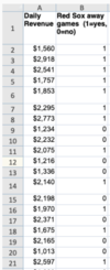
The owner of Boston sports bar believes that, on average, her restaurant is busier on days when the Red Sox play an away game (a game played at another team’s stadium), but she wants to be sure before adding more staff. To test whether this is true, she takes a random sample of 50 days over the course of the baseball season and records the total daily revenue, along with whether the Red Sox were playing away that day (1 if yes, 0 if no). Using the data provided, perform a regression analysis to determine the effect of Red Sox away games on revenue. Be sure to include the residuals and residual plot in your analysis.

A

From the Data menu, select Data Analysis, then select Regression. The Input Y Range is A1:A51 and the Input X Range is B1:B51. You must check the Labels box to ensure that the regression output table is appropriately labeled. You must also check the Residuals and Residual Plots boxes so that you are able to analyze the residuals.

29
Q

The sports bar owner runs a regression to test whether there is a relationship between Red Sox away games and daily revenue. Which of the following statements about the regression output is true? SELECT ALL THAT APPLY.

  • The average daily revenue for days when the Red Sox do not play away is $1,768.32.
  • The average daily revenue for days when the Red Sox play away is $1,768.32.
  • The average daily revenue for days when the Red Sox play away is $2,264.57.
  • The average daily revenue for days when the Red Sox do not play away is $1,272.07.
  • On average, the bar’s revenue is $496.25 higher on days when the Red Sox play away than on days when they do not.
A

The average daily revenue for days when the Red Sox do not play away is $1,768.32.

This option is true. $1,768.32 is the average daily revenue on days when the Red Sox do not play away.

The average daily revenue for days when the Red Sox play away is $1,768.32.

This option is false. The average daily revenue on days when the Red Sox play away is $1,768.32+496.25=$2,264.57.

The average daily revenue for days when the Red Sox play away is $2,264.57.

This option is true. The average daily revenue on days when the Red Sox play away is $1,768.32+496.25=$2,264.57.

The average daily revenue for days when the Red Sox do not play away is $1,272.07.

This option is false. $1,768.32 is the intercept which represents the average daily revenue when “Red Sox”=0 (that is, a day when the Red Sox do not play away).

On average, the bar’s revenue is $496.25 higher on days when the Red Sox play away than on days when they do not.

This option is true. When “Red Sox away game”=1, you must add the coefficient for Red Sox away game to the intercept. Therefore, on average, revenue is $496.25 higher on days when the Red Sox play away than on days when they do not.

30
Q

The sports bar owner runs a regression to test whether there is a relationship between Red Sox away games and daily revenue. Based on the regression output below, what proportion of the variability in revenue can be accounted for by whether the Red Sox are playing away.

Please enter the value of the percentage with ONE digit to the right of the decimal place. For example, if you think that 96.6925% of the variability is explained, enter 96.7.

Number:

A

The R Square value measures how much of the total variation in the dependent variable (in this case, revenue) that is explained by the independent variable (in this case, away game). As shown in the regression output, the R-square value is 0.2252, or approximately 22.5%

31
Q

Is the relationship between Red Sox away games and average daily revenues significant at the 95% confidence level? Choose the correct answer with the corresponding correct reasoning.

  • No, because R Square is less than 50%
  • Yes, because the slope is positive.
  • Yes, because the p-value of the intercept is less than 0.05
  • Yes, because the p-value of the intercept is less than 0.95
  • Yes, because the p-value of the independent variable is less than 0.05
  • Yes, because the p-value of the independent variable is less than 0.95
A

No, because R Square is less than 50%

R Square indicates the explanatory power of a regression model, but does not indicate whether the relationship is significant.

Yes, because the slope is positive.

The slope does not indicate whether the relationship is significant.

Yes, because the p-value of the intercept is less than 0.05

The p-value of the intercept does not indicate whether the relationship is significant.

Yes, because the p-value of the intercept is less than 0.95

The p-value of the intercept does not indicate whether the relationship is significant.

Yes, because the p-value of the independent variable is less than 0.05

Since the p-value, 0.0005, is less than 0.05, we can be confident that the relationship is significant at the 5% significance level and, equivalently, at the 95% confidence level.

Yes, because the p-value of the independent variable is less than 0.95

The relationship is significant at the 95% confidence level, but not because the p-value is less than 0.95. For a relationship to be significant at the 95% confidence level, the p-value must be less than 0.05, the 5% significance level.

32
Q

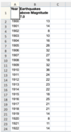
A scientist believes that, over the years, the number of major earthquakes has been decreasing. To test his hypothesis, the scientist collects data on the number of earthquakes above magnitude 7.0 on the Richter scale that have occurred each year from 1900 to 2012. Using the data below create a scatter plot with year on the horizontal axis.

A

From the Insert menu, select Scatter, then select Scatter With Only Markers. The Input Y Range is B1:B114 and the Input X Range is A1:A114. You must check the Labels in first row box to ensure that the scatter plot’s axes are appropriately labeled.

33
Q

Here is the scatter plot based on the earthquake data from 1900 to 2012. Which of the following are true about large (greater than 7.0 magnitude) earthquakes, based on the plot? SELECT ALL THAT APPLY.

  • The most earthquakes occurred in the 1940s.
  • There were about 50 earthquakes in the year with the most earthquakes.
  • There were about 6 earthquakes in the year with the least earthquakes.
  • The number of earthquakes appears to be decreasing.
  • The year with the most earthquakes has about 20 more earthquakes than the year with the least earthquakes.
A

The most earthquakes occurred in the 1940s.

The year with the most earthquakes is indicated by the highest point on the graph. This point is above and slightly to the right of the marker for 1940 and the next few years also have high numbers of earthquakes.

There were about 50 earthquakes in the year with the most earthquakes.

The top value on the y-axis is 50, but the highest data point is only a little more than 40.

There were about 6 earthquakes in the year with the least earthquakes.

Looking at the graph, there are several years in the early 1900s and in the 1980s with less than 10 earthquakes. The year with the least number of earthquakes falls in the mid-1980s. The marker for that year is at about 6, between the lines at zero and 10 earthquakes.

The number of earthquakes appears to be decreasing.

We can see by the downward slope of the line that the number of earthquakes decreases slightly over time.

The year with the most earthquakes has about 20 more earthquakes than the year with the least earthquakes.

The year with the most earthquakes has more than 35 more earthquakes than the year with the least earthquakes.

34
Q

The scientist performs additional analyses and observes that the number of major earthquakes does appear to be decreasing but wonders whether the relationship is statistically significant. Based on the partial regression output below and a 5% significance level, is the year statistically significant in determining the number of earthquakes above magnitude 7.0?

  • Yes
  • No
  • The answer cannot be determined without further information
A

Yes

Since the p-value is not provided, the confidence interval for the coefficient should be used. Since the 95% confidence interval, -0.11 and -0.04, does not contain zero, the coefficient for year is statistically significant.

No

See correct answer for explanation.

The answer cannot be determined without further information

See correct answer for explanation.

35
Q

Based on the scientist’s regression model, forecast the number of earthquakes above magnitude 7.0 that will occur in 2019.

A

The expected number of earthquakes above magnitude 7.0 that will occur in 2019 is B15+B16*2019=14.4. You must link directly to values in order to obtain the correct answer.

36
Q

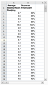
A researcher at a university wants to better understand how study habits affect student grades. To determine whether there is a link between hours spent studying and exam scores, the researcher recruits fifty students in an advanced calculus class to record their study hours over the semester, and also obtains permission to see their scores on the final exam. Perform a regression analysis, where the average number of hours spent studying per week over the two-month data collection period is the independent variable and the score on the final exam is the dependent variable. Be sure to include the residuals and residual plot in your analysis.

A

From the Data menu, select Data Analysis, then select Regression. The Input Y Range is B1:B51 and the Input X Range is A1:A51. You must check the Labels box to ensure that the regression output table is appropriately labeled. You must also check the Residuals and Residual Plots boxes so that you are able to analyze the residuals.

37
Q

What is the correlation coefficient of the relationship between the average weekly hours spent studying and the score on the final exam?

  • 0.7105
  • 0.2394
  • 0.2549
  • 0.5049
A
  1. 7105
  2. 7105 is the square root of the Multiple R value.
  3. 2394
  4. 2394 is the Adjusted R2 value.
  5. 2549
  6. 2549 is the R2 value.

0.5049

0.5049 is the Multiple R value. Remember that for single variable linear regression, Multiple R, which is the square root of R2, is equal to the absolute value of the correlation coefficient. The regression coefficient for Average Weekly Hours Studying (0.03, as shown in the bottom table of the output) is positive, so the slope is of the regression line is positive. Therefore, the correlation coefficient must also be positive.

38
Q

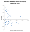
Based on the residual plot, do you think that this regression model is a good fit?

  • Yes
  • No
A

Yes

The linear model does not appear to be a good fit because the residuals are not randomly distributed. The residuals form a funnel shape, which indicates that they are heteroskedastic.

No

The linear model does not appear to be a good fit because the residuals are not randomly distributed. The residuals form a funnel shape, which indicates that they are heteroskedastic. That is, the size of the residuals grows (in absolute value) as the average weekly hours studying decreases.

39
Q

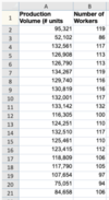
A human resources department wants to understand the relationship between the number of factory workers and production volume, which is measured in units produced per day. Perform a regression analysis, where the number of workers is the independent variable and production volume is the dependent variable. Be sure to include the residuals and residual plot in your analysis.

A

From the Data menu, select Data Analysis, then select Regression. The Input Y Range is A1:A21 and the Input X Range is B1:B21. You must check the Labels box to ensure that the regression output table is appropriately labeled. You must also check the Residuals and Residual Plots boxes so that you are able to analyze the residuals.

40
Q

How much variation in production volume can be explained by the number of factory workers?

  • 55.21%
  • 57.56%
  • 75.87%
  • 0.01%
A
  1. 21%
  2. 21% is the Adjusted R2 value.

57.56%

The percent of variation in production volume that can be explained by the number of factory workers is represented by the R2 value. The R2 value is 57.56%.

  1. 87%
  2. 87% is the Multiple R value.
  3. 01%
  4. 01% is the p-value of the slope.
41
Q

What is the expected change in production volume, on average, as the number of factory workers decreases by five?

Please enter the value of the expected change in production volume with ONE digit to the right of the decimal place. For example, if you think the expected change in production volume is a DECREASE of 100.75, enter -100.8. _________

Number:

A

Since the slope represents the average change in production volume as the number of factory workers increases by one, the average change in production volume as the number of factory workers decreases by five is 1,638.98(-5)=-8,194.9.

42
Q

Based on the regression model, forecast the expected production volume when there are 112 factory workers.

A

The expected production volume when there are 112 factory workers is B15+B16*112=118,846. You must link directly to values in order to obtain the correct answer.

43
Q

Based on the regression model, the expected daily production volume with 112 factory workers is 118,846 units. The human resource department noted that 123,415 units were produced on the most recent day on which there were 112 factory workers. What is the residual of this data point?

  • -4,569 units
  • -2,163 units
  • -41 units
  • 41 units
  • 2,163 units
  • 4,569 units
A

4,569 units

The residual is equal to the historically observed value minus the regression’s predicted value(ε=y-ŷ). 112 factory workers historically produced 123,415 units, whereas the regression model predicts that 112 workers would produce 118,846 units. The residual is the difference between these two values: 123,415 units – 118,846 units = 4,569 units.

44
Q

If the expected production volume when there are 120 workers is approximately 131,958 units, which of the following equations would provide a reasonable estimate of the 68% prediction interval for the output of those 120 workers?

  • 120±14,994.93
  • 131,958±14,994.93
  • 131,958±29,989.56
  • 120±331.69
  • 131,958±331.69
  • 131,958±663.38
A

120±14,994.93

The value of the independent variable is not the center of the prediction interval.

131,958±14,994.93

A reasonable estimate of the prediction interval is the point forecast (131,958) plus or minus the z-value times the standard error of the regression (14,994.93). As usual, the z-value is based on the desired level of confidence. Since we want a 68% prediction interval, the z-value is equal to one. Therefore 131,958±14,994.93 is the best option.

131,958±29,989.56

This would be a good estimate of the 95% prediction interval, for which the z-value would be approximately 2. For a 68% prediction interval, the z-value is one.

120±331.69

The value of the independent variable is not the center of the prediction interval. Also, the prediction interval uses the standard error of the regression model, which is 14,994.93, not the standard error of the slope.

131,958±331.69

The prediction interval uses the standard error of the regression model, which is 14,994.93, not the standard error of the slope (331.69).

131,958±663.38

The prediction interval uses the standard error of the regression model, which is 14,994.93, not the standard error of the slope. Also, for a 68% prediction interval, the z-value is equal to one.

45
Q

Below is a partial regression output table, which of the following values most likely belongs in the Lower 95% cell for the independent variable in the output table?

  • -6.01
  • -2.45
  • 1.78
  • 2.45
  • The answer cannot be determined without further information
A

-6.01

Since the p-value, 0.3956, is greater than 0.05, the linear relationship is not significant at the 95% confidence level. Therefore, the 95% confidence interval of the slope must contain zero. The confidence interval is centered around the slope of 1.78, so the lower and upper bounds must be equally distant from the slope. The slope, 1.78, is not in the middle of -6.01 and 6.01.

-2.45

Since the p-value, 0.3956, is greater than 0.05, the linear relationship is not significant at the 95% confidence level. Therefore, the 95% confidence interval of the slope must contain zero. The confidence interval is centered around the slope of 1.78, so the lower and upper bounds must be equally distant from the slope. The Upper 95% minus the slope is 6.01–1.78=4.23, so the Lower 95% is 1.78–4.23=-2.45.

  1. 78
  2. 78 is the predicted value of the coefficient. The confidence interval must be centered on 1.78.
  3. 45

Since the p-value, 0.3956, is greater than 0.05, the linear relationship is not significant at the 95% confidence level. Therefore, the 95% confidence interval of the slope must contain zero. The interval between 2.45 and 6.01 does not contain zero.

The answer cannot be determined without further information

The Lower 95% can be found by calculating the difference between the Upper 95% and the slope, then subtracting that difference from the slope.

46
Q

The scatter plot below displays the relationship between two variables. Which of the following options most accurately describes the R-squared value and the p-value of this relationship?

  • High R2; high p-value (i.e., p-value greater than 0.05)
  • High R2; low p-value (i.e., p-value less than 0.05)
  • Low R2; high p-value (i.e., p-value greater than 0.05)
  • Low R2; low p-value (i.e., p-value less than 0.05)
A

High R2; high p-value (i.e., p-value greater than 0.05)

A high R2 and high p-value indicates that the independent variable explains a lot of the variation in the dependent variable but the linear relationship is not significant.

High R2; low p-value (i.e., p-value less than 0.05)

A high R2 and low p-value indicates that the independent variable explains a lot of the variation in the dependent variable and the linear relationship is significant.

Low R2; high p-value (i.e., p-value greater than 0.05)

A low R2 and high p-value indicates that the independent variable explains little variation in the dependent variable and the linear relationship is not significant. Since the data points are widely dispersed and do not indicate a clear linear pattern, this relationship likely has a low R2 and high p-value.

Low R2; low p-value (i.e., p-value less than 0.05)

A low R2 and low p-value indicates that the independent variable explains little variation in the dependent variable but the linear relationship is significant.