HW 1

Question 1

What is the average wage gap between blacks and nonblacks in this model?

Answer 1

The UNCONDITIONAL log wage gap is -0.318. I.e. blacks have a

(e^-0.318-1) * 100% = -27.2%

lower wage than nonblacks on average.

Question 2

What is the average wage gap between blacks and nonblacks in this model?

Answer 2

The CONDITIONAL log wage gap is

-0.178 = (e^-0.178-1) * 100% = -16.3%

lower wages.

Question 3

Give an economic explanation as to why the estimated
gaps di er between the models. What do you conclude concerning underspecification and possible endogeneity problems?

Answer 3

Part of the unconditional difference is driven by fact that wage also depends on education, experience, and region. The gap is smaller in the second model, because blacks are more likely to have less education, experience and live in the south.

The first model is clearly underspecified, as important predictor variables for the wage were omitted. Since these omitted variables are correlated with “black”, the effect of “black” in model1 is biased.

Question 4

Model 3 additionally includes interaction terms between black and experience and experience squared to analyze whether the racial wage gap depends on experience. Calculate the average wage gap between blacks and non-blacks for workers with x years of experience.

Answer 4

difference calculation (calculate only the terms that are multiplied with “black”, as only these differ):

0.15989 + exper*-0.0541 + exper² * 0.00164

Question 5

Explain the idea of AIC and the role of the two components of the AIC formula.

Answer 5

• Idea: bias-variance tradeoff, more parameters decrease bias but increase variance
• RSS(K): As K increases, RSS decreases -> less bias. This rewards the quality of the approcimation
• 2K/N: As K increases, variance increases. This part “punishes” simply adding additional parameters.

Question 6

What are the advantages of the AIC compared to R2 for the purpose of model selection?

Answer 6

The R2 only cares about the bias, and thus always suggests the model with the largest number of parameters. The AIC is better because it weights bias and variance against each other.

Question 7

Based on the results, which model do you prefer?

Answer 7

Model 3 performs best (lowest AIC) and is therefore preferable.

Question 8

Show theoretically that OLS regression residuals are in general not homoskedastic, even if the error terms are homoskedastic.

Answer 8

1. Bring residuals in appropriate form:
   e = Y - X^β = Y - X(X’X)^-1X’Y = (I_N - P) Y
2. Detect distribution (homo- or heteroskedastic):
   Var(e) = Var( (I_N - P) Y ) = (I_N - P) Var(Y) (I_N - P)’ =
   = M Var(ε) M’ = M σ²I_N M’
3. As M is the residual maker and idempotent so that MM’ = M: Var (e) = (I_N - P) σ²I_N
4. From (I_N - P) we see that residuals are generally not homoskedastic

Question 9

Explain how you would use residual analysis to check for heteroskedasticity.

Answer 9

Transform the residuals to standardized or studentized residuals and plot against fitted values.

Question 10

How can the OLS regression residuals be transformed in an appropriate way to detect heteroskedasticity graphically?

Answer 10

1. We know that OLS residuals have Var(e_i) = (1 - P_ii)σ²
2. Standardized residuals are defined by:
   * *ẽ_i = e / [σ√(1-p_ii)]**
3. Therefore the variance of standardized residuals is:
   * *Var(ẽ_i) = [1 / σ√(1-p_ii)] Var(e_i) [1 / σ√(1-p_ii)]’**
4. Through simplification, you get Var(ẽ_i) = 1

Question 11

Explain how the White test for heteroskedasticity is implemented.

Answer 11

• H₀: E [e_i² | x_i] = σ² = constant
• H₁: E [e_i² | x_i] ≠ constant

Regress squared OLS residuals on all variables from the linear model (incl. interaction term and squares), intercept is the constant variance. Under H₀, the regressors should be jointly insignificant.

Question 12

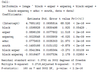
The results of the White test for model 3 are given in the output. How do you interpret the result of the test? What do you conclude?

Answer 12

p-value = 0.093

At 5% significance, we fail to reject H₀ (homoskedasticity).

At 10% significance, we reject H₀ (homoskedasticity).

Question 13

What is the interpretation of the coefficient on cigpacks?

Answer 13

Each additional pack of cigaretts decreases the birth weight by 11.5 ounces, holding the other variables fixed. The effect is statistically significant at the 1%-level.

Question 14

Under which condition is the OLS estimator of the effect of cigpacks unbiased? Under which condition is it consistent? Do you think these conditions are fulfilled in the given example?

Answer 14

• Condition for unbiasedness: E(ε|X)=0
• Condition for consistency: E(X’ε) = 0 or Cov(ε, X)=0

Conditions are likely not fulfilled. There could be some unobserved characteristics of the mother (e.g. health, personality traits etc.) that affect both smoking during pregnancy and the child’s weight.

Question 15

Which two conditions have to be fulfilled for an instrument to be valid? Can these conditions be tested, and if yes, how?

Answer 15

1. RELEVANCE of the instrument: Cov (X, Z) ≠ 0
   - -> Can be tested by regressing X on Z (and all other variables to check if the effect on Z is significant
2. EXOGENEITY of the instrument: E(ε_i‘z) = 0
   - -> Can not be tested

Question 16

In the present example, we use the variable cigprice as an instrument for cigpacks. Interpret the results below. Do you think cigprice is a suitable instrument in this context? Can you identify problems in the IV estimation of this example?

Answer 16

Instrument is not statistically significant (p-value 0.317), i.e. the cigarette price has no effect on cigarette consumption.

–> The “relevance” condition for the instrument is clearly not fulfilled, and the instrument should not be used!

Question 17

In the present example, we use the variable cigprice as an instrument for cigpacks. Interpret the results below. Do you think cigprice is a suitable instrument in this context? Can you identify problems in the IV estimation of this example?

Answer 17

• One additional pack increases (!) the birth weight by 70.8 ounces, ceteris paribus.
• Effect is not statistically significant.
• Result is unexpected: positive sign and very large magnitude. The IV estimation is highly suscept given the weak instrument in the First Stage.

–> This is an example that weak instruments can sometimes produce extreme results.

Question 18

What is the purpose of the Hausman test in the case of IV estimation? In the present example, the Hausman test gives a p-value of 0.278. Interpret this result. What are the limitations of the Hausman test in the present example?

Answer 18

Wu-Hausmann test tests whether variable is actually exogenous:

• H₀: cigpacks is exogeneous, H₁: cigpacks is endogenous
• p-value of 0.272 –> Fail to reject the H0 of exogeneity, i.e. there is no evidence that there is an endogeneity problem. OLS is consistent.

LIMITATIONS:

• Assumes that the instrument is valid
• May fail to reject H₀ if standard errors are high

Question 19

Assume that the data are generated according to the first model below, but we estimate the coefficient of x on the basis of the second model. What are the necessary steps to show the bias of the OLS estimator ^β?

Answer 19

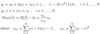
1. Get rid of the intercept by defining the residual maker P₀ = X(X’X)^-1X’ (in this case, X = 1_N)
2. Transform the model by multiplying each component with the residual maker M₀ = I_N - P₀
3. Calculate the bias (^β) = E [^β] - β₀
   
   • Use that E [^β] = E[(X’X)^-1X’Y]

Question 20

How is the residual maker M defined?

Answer 20

M = I - P = I - X(X’X)^-1X’

Question 21

How can you rewrite the average of y = ȳ as a sum?

Answer 21

1/N Σ_i=1^N y_i

Question 22

What is |m|?

Answer 22

the number of model parameters = k

Question 23

What is the average of p_ii?

Answer 23

avg(p_ii) = 1/N Σ_i=1^N p_ii =1/N tr(P) = 1/N tr(I_k) = K/N

Question 24

Which model would you choose? Discuss first whether it is possible to compare all three models by the given AIC values.

Answer 24

The three models cannot directly be compared:

• the first two are normally distributed, but
• the third assumes a normal distribution for log(y)

Of the first two, I’d choose the first which has a lower AIC.

Question 25

How can this sum be simplified?

^∞Σ_j=0 β^jρ^j

Answer 25

^∞Σ_j=0 β ^j ρ ^j =

= ^∞Σ_j=0 (βρ) ^j =

= 1 / (1 - βρ)

Question 26

Can β be estimated by OLS in this case? Why?

Answer 26

No: E [ε_t, y_t-1] ≠ 0

β will thus not be consistent - unless ρ = 0 or σ_v² = 0

Question 27

Can β be estimated by OLS in this case? Why?

Answer 27

Yes:

the error term v_t is iid and y_t-1, y_t-2 are predetermined, thus:

E [y_t-1, v_t] = 0 and OLS is appropriate