HBX- BA - 5 Flashcards

15%
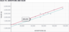
The R2 value is approximately 0.15, or 15%. This means that 15% of the variation in selling price is explained by a home’s distance from Boston.
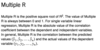
Multiple Regression (two or more independent variables) - Equation & Explanation
We use multiple regression to investigate the relationship between a dependent variable and multiple independent variables.
For multiple regression we rely less on scatter plots and more on numerical values and residual plots because visualizing three or more variables can be difficult.
Forecasting with a multiple regression equation is very similar to forecasting with a single variable linear model. However, instead of entering only one value for a single independent variable, we input a value for each of the independent variables.

Gross Relationship
The relationship between a single independent variable and a dependent variable. The gross relationship is affected by any variables that are related to the independent and/or dependent variable but are not included in the model.
In the graph below Because we are not considering any other factors
in this regression, we call this the gross effect of distance on price.
**We interpret the distance coefficient as meaning that
on average, prices decrease by $15,163 for each additional mile
a house is from Boston.

Net Relationship
A relationship between an independent variable and a dependent variable that controls for other independent variables in a multiple regression. Because we can never include every variable that is related to the independent and dependent variables, we generally consider the relationship between the independent & dependent variables to be net with regard to the other independent variables in the model, and gross with regard to variables that are not included.
CAN BE CALLED EITHER: net effect of distance on price or as the effect of distance on price controlling for house size.
The graph below tells us that for every additional mile a house is from Boston, on average price decreases by $10,840, assuming that the size of the house stays the same.
Multiple Regression Continued….
In Singular Regression - the variables being studied sometimes take on the effects of other variables. When they are separated in multiple regression, they’re able to be free and reflect their true values! (If we’ve included everything)
This also affects the equation (since there are so many variables) …
A coefficient is net with respect to all variables included in the model, but gross with respect to all omitted variables. It’s important to always keep in mind that included variables may be picking up the effects of omitted variables–
Which model would we use to predict the price of a house that is 2,700 square feet?
- SellingPrice=194,986.59+244.54(HouseSize)−10,840.04(distance from Boston)
- SellingPrice=13,490.45+255.36(HouseSize)
- SellingPrice=686,773.86–15,162.92(distance from Boston)
SellingPrice=13,490.45+255.36(HouseSize)
- Since we have data about just one independent variable, we should use a single variable regression model. This is a single variable linear regression model, in which house size is the only independent variable.
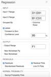
Suppose we want to forecast selling price based on house size and distance from Boston. Which equation should we use to forecast the price of a house that is 2,700 square feet and 15 miles from Boston?
- SellingPrice=194,986.59+244.54(HouseSize)–10,840.04(distance from Boston)
- SellingPrice=13,490.45+255.36(HouseSize)SellingPrice=13,490.45+255.36(HouseSize)
- SellingPrice=686,773.86–15,162.92(DistancefromBoston)
SellingPrice=194,986.59+244.54(HouseSize)–10,840.04(distance from Boston)
- Since we have data about two independent variables, house size and distance from Boston, we should use the multiple regression model with those two variables.
The expected selling price of a 2,700 square foot home that is 15 miles from Boston is B2+B3*2700+B4*15=$692,646.51. You must link directly to the values in order to obtain the correct answer.
Two houses are the same size, but located in different neighborhoods: House B is five miles farther from Boston than House A. If the selling price of House A was $450,000, what would we expect to be the selling price of House B?
SellingPrice=194,986.59+244.54(HouseSize)–10,840.04(DistancefromBoston)
SellingPrice=13,490.45+255.36(HouseSize)
SellingPrice=686,773.86–15,162.92(DistancefromBoston)
Approximately $396,000
Since the two houses are the same size, to predict the expected difference in selling prices we should use the net effect of distance on selling price (that is, the effect of distance on selling price controlling for house size). This value, -$10,840.04/mile, is found in the multiple regression model. House B is five miles farther from Boston than House A so House B’s expected selling price is: =House A’s selling price+net effect of distance on selling price≈$450,000–$10,840.04(5miles)≈$450,000–$54,200.20≈$395,799.80

Price
We are trying to estimate the price of the TV, so PricePrice is our dependent variable.

- 55
- 55 is the coefficient for PictureQualityPictureQuality.
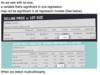
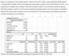
The expected selling price of a 1,500 square foot home that is 10 miles from Boston is B15+B16*1,500+B17*10=$453,397.59. You must link directly to the values in order to obtain the correct answer.
Assume we have created two single linear regression models, and a multiple regression model to predict selling price based on House Size alone, Distance from Boston alone, or both. The three models are as follows, where House Size is in square feet and distance from Boston is in miles:
SellingPrice=13,490.45+255.36(HouseSize)
SellingPrice=686,773.86–15,162.92(distance from Boston)
SellingPrice=194,986.59+244.54(HouseSize)–10,840.04(distance from Boston)
House A and House B are the same size, but located in different neighborhoods: House B is five miles closer to Boston than House A. If the selling price of House A is $450,000, what would we expect to be the selling price of House B?
Approximately $504,000
Since the two houses are the same size, to predict the expected difference in selling prices we should use -$10,840.04/mile, the net effect of distance on selling price (that is, the effect of distance on selling price controlling for house size), which can be found in the multiple regression model. House B is five miles closer to Boston than House A so House B’s expected selling price is: House A’s selling price+net effect of distance on selling price ≈ $450,000+$10,840.04(5 miles) ≈ $450,000+$54,200.20 ≈ $504,200.20
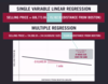
In single variable regression, to measure the predictive power of a single independent variable we used R2 : the percentage of the variation in the dependent variable explained by the independent variable. For multiple regression models, we will rely on ______
Adjusted R2
Adjusted R2
A measure of the explanatory power of a regression analysis.
Adjusted R-squared = R-squared multiplied by an adjustment factor that decreases slightly as each independent variable is added to a regression model.
Unlike R-squared, which can never decrease when a new independent variable is added to a regression model, Adjusted R-squared drops when an independent variable is added that does not improve the model’s true explanatory power. Adjusted R2 should always be used when comparing the explanatory power of regression models that have different numbers of independent variables.
***R2 can only stay the same or increase. —> This is why we need Adjusted R2
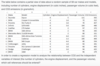
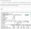
In the case below, since the adjusted R-squared of the multiple regression
of price versus house size and distance is greater than the adjusted R-squared of either single variable regression, we can conclude that we gained real explanatory power by incorporating both independent variables
How should single variable regression models and multiple regression models be interpreted?
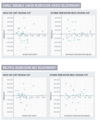
Recall that residuals represent the differences between the actual and predicted values of the dependent variable (selling price in this case).
The house size residual plots for multiple and single variable linear regression represent different quantities:
- the residual plot for the single variable regression gives us insight into the gross relationship between price and house size;
- and the residual plot for multiple regression gives us insight into the net relationship between price and house size, controlling for distance.
The residual plots for the independent variable distance from Boston (the two plots on the right side in the panel) should be interpreted similarly:
- the residual plot for single variable regression gives us insight into the gross relationship between price and distance;
- and the residual plot for multiple regression gives insight into the net relationship between price and distance, controlling for house size.
P-Value + Multiple Regression
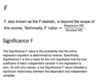
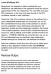
As in single variable linear regression, we must inspect the p-value of each independent variable to assess whether its relationship with the dependent variable is significant.
If the p-value is less than 0.05 for each of the independent variables, we can be 95% confident that the true coefficients of each of the independent variables are not zero. In other words, we can be confident that there is a significant linear relationship between the dependent variable and the independent variables.

Yes
Since the p-value for the independent variable (house size), 0.0000, is less than 0.05, we can be confident that the relationship between price and house size is significant. Recall that the p-value for the intercept does not determine the significance of the relationship between the dependent and independent variable, so even though the p-value for the intercept is greater than 0.05, we can still say that the relationship between price and house size is significant.
Yes
The p-values for the independent variables (house size and distance), 0.0000 and 0.0033, respectively, are less than 0.05, so we can be confident that the relationship between price, house size, and distance is significant.
What are the metrics to determine whether a multiple variable linear regression model is a good fit for our data.
1.)) Because R2 never decreases when independent variables are added to a regression, it is important to multiply it by an adjustment factor when we assess the fit of a multiple regression model. This adjustment factor compensates for the increase in R2 that results solely from increasing the number of independent variables.
-
Adjusted R2 is provided in the regression output.
It is particularly important to look at Adjusted R2, rather than R2, when comparing regression models with different numbers of independent variables.
2.)) In addition to analyzing Adjusted R2, we must test whether the relationship between the dependent variable and independents variables is linear and significant. We do this by analyzing the regression’s residual plots and the p-values associated with each independent variable’s coefficient.
- For multiple regression models, residual plots are an indispensable tool for detecting whether the linear model is a good fit.
- We rely heavily on residual plots for multiple regression models because the full relationship among multiple independent variables and the dependent variable is difficult or impossible to represent in a single scatter plot. (When there are two independent variables, the regression model describes the best fit plane through the data and the residuals can be seen on the three-dimensional scatter plot as well as on their individual residual plots.)
- The residuals are the difference between the historically observed values and the values predicted by the regression model.
- There is a residual plot for each independent variable included in the regression model.
- We can graph a residual plot for each independent variable to help detect patterns such as heteroskedasticity and nonlinearity.
- As with single variable regression models, if the underlying multiple relationship is linear, the residuals follow a normal distribution with a mean of zero and fixed variance.
- We should also analyze the p-values of the independent variables to determine whether there is a significant relationship between the variables in the model. If the p-value of each of the independent variables is less than 0.05, we conclude that there is sufficient evidence to say that we are 95% confident that there is a significant linear relationship between the dependent and independent variables.
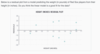
Yes, this looks like a linear relationship.
There is nothing in this scatterplot to concern us.
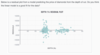
No, there is heteroskedasticity.
There is evidence of heteroskedasticity; there is more variability at the lower values than at the higher values.
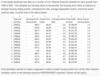
- Runs
- Strikeouts
- Completed Games
- ERA
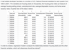
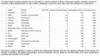
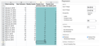
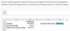
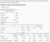
The p-value column in the bottom table gives the significance level of each variable. The only p-values that are less than .05 are for the Intercept (which we do not assess for significance) and ERA. Thus, ERA is the only independent variable that is significant at p < .05. Note also that ERA is the only independent variable with a 95% confidence interval that does not contain 0.
Significant: ERA
Not significant: Runs, Strikeouts, Completed Games
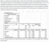
- 0%
- 6298 or 63.0% is the R-square, which indicates how much variability is accounted for by the model.