Factor Analysis Flashcards
(29 cards)
First stage of factor analyis
Most require a matrix of product-moment correlation coefficients as the basic data input. The alternatives are between those matrices based on correlations between different variables, or of taking a matrix of correlation coeffficients measuring the degree of similarity between a set of individuals based on a number of variables or attributes.
Correlation matrix of selected variables
Called R-mode factoring. Concerned at looking at the degrees of similarity between the areas and to distinguish spatially-based, rather than variable-based, arrangements and groupings.
Areas which show correlation
Pairs of areas, which have similar attributes, will display a strong positive correlation, and those pairs with contrasting values across the variables will have a strong negative correltion. This is referref to as Q-mode factoring.
The second stage
Known as factor extraction - to explore the possibilities of data reduction by constructing a new, and smaller, set of variables based on the interrelationships in the correlation matrix.
Two approaches to the second stage
Principal component analysis and factor analysis. In both of these strategies, new variables are defined as mathermatical transformations and combinations of the original data.
Factor analysis model
The assumption is made that the correlations are largely the result of some underlying regularity in the basic data. Specifically, it assumes the behaviour of each original variable is partly influenced by the various factors that are common to all the variables.
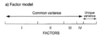
Common and unique variance
The degree to which there are various factors common to all variables is termed the common variance, where as the unique variance is an expression of the variance that is specific to the variable itself and to errors in its measurement.
Principal components analysis
Cocnerned with describing the variation or variance that is shared by the data points on three or more variables. Makes no assumptions about the structure of the original variables. It does not presuppose any element of unique variance to exist within each variable, and the variances are assumed to be entirely common in character.
Principal component analysis stages
1 - communalities - assumed to be 1, the extraction column indicates the degree of common variance to each variable after the analysis is complete. 2 - Initial eigenvalues - “eigenvalue” is the amount of variance they account for. 3 - Extraction sums - first three factors collectively account for nearly 72% of the total variance
Principal component analysis - factors to retain/reduction of variables
The point is to reduce the number of variables. Two ways to do this: Using Kaiser’s criterion to select those features that have an eigen value greater than one; and scree test (Catell, 1966) - looking for the flattening of the slope.
Final stage in which variations in the method are possible in the search of interpretable factors.
The point at which we analyse the character of the factors and qualities that they represent. We might choose to refine or clarify the factor model, through factor rotation. This involves rotating the axes as fixed set in n-dimensional space in order to account for the greater degree of the original data.
Rotation of axes
We may rotate axes independently so that they become oblique to one another. This may increase the utility of factoring model, but a degree of correlation will now exist between the different, now non-orthogonal, factor axes.
Two types of rotation of axes
1 - Orthogonal rotation - produces factors that unrelated to or independent of one another. 2 - Oblique rotation - in which the factors are correlated.
Two theoretical approaches
One based on algebraic solutions and the second based on geometric intepretations
Simple correlation
Had the points fallen perfectly along a striaght line the correlation would have been +1.0. On the other hand, had there been no correlation between the two variables the points would have formed a vaguely circular scatter on the graph with no apparent trend.
Simple correlation from the point of view of geometry
The two extremes - the perfect and the zero correlation - represent the two limiting conditions between which all other states will plot on the graph in the form of ellipsoidal scatters of points with varying degrees of two extreme cases together with an intermediate condition. The latter in particular draws attention to the important point that all such ellipses can be described by reference to a major and minor axis.
Major axis can be viewed as representing
The common variance between the two variables and is in some ways comparable to a regression line.
The minor axis
More akin to the residual variance. Thus, when we have a perfect relationship the major axis is at its greatest length and the minor axis disappears.
The lengths of axis can be determined and estimated by
They can be determined by computer programs in which the axes, or eigenvectors, are estimated and their statistical length measured by what is termed their eigenvalue.
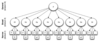
Spearman’s two factor intelligence theory
Each small oval is a hypothetical mental test. The blue areas correspond to test-specific variance, while the purple areas represent the variance attributed to g.

John B. Carroll’s three stratum theory
A model of cognitive abilities. The broad abilities recognized are fluid intelligence (Gf), crystallized intelligence (Gc), broad visual perception (Gv) etc. Carrol regarded the broad abilities as “flavours” of g.
Analysis of dependence
In which one variable is identified for study and is then examined in terms of its dependence on others.
Analysis of interdependence
The interdependence that might exist between all variables with no reference to any particular one of them being ‘dependent’.
Used to address multicollinearity
If variables are related because they are related to underlying factors controlling Y, they may be reduced using factor or principal component analysis.
