Chapter 5: Joint Probability Distributions Flashcards

1
Q

Joint Probability Mass Function for Discrete Variables

A
2
Q

Joint Probability Mass Function for Continuous Variables

A
3
Q

Joint Probability Density Function for Continuous Variables

A
4
Q

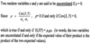
Example of Joint Probability Density

A
5
Q

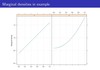
Marginal Densities in example

A
6
Q

Independent Random Variables

A
7
Q

Independent Random Variables Explained

A
  • The definition says that two variables are independent if their joint pmf or pdf is the product of the two marginal pmf’s or pdf’s.
  • Intuitively, independence says that knowing the value of one of the variables does not provide additional information about what the value of the other variable might be.
  • Independence of X and Y requires that every entry in the joint probability table be the product of the corresponding row and column marginal probabilities.
  • Independence of two random variables is most useful when the description of the experiment under study suggests that X and Y have no effect on one another.
    • Then once the marginal pmf’s or pdf’s have been specified, the joint pmf or pdf is simply the product of the two marginal functions. It follows that
8
Q

Conditional Distributions

A
9
Q

Expected Value

A
10
Q

Covariance

A
  • Thus, the covariance of and provides a measure of the degree to which two variables X and Y tend to “move together”:
    • a positive covariance indicates that the deviations of X and Y and from their respective means tend to have the same sign;
    • a negative covariance indicates that deviations of X and Y from their respective means tend to have opposite signs.
11
Q

Correlation

A
12
Q

Correlation Coefficient

A
13
Q

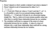
Properties of the Correlation Coefficient

A
14
Q

Joint PMF of Two Discrete Random Variables

A
15
Q

Marginal PMF of Two Discrete RVs

A
16
Q

Example: Joint Probability Distribution of 2 Discrete RVs

A
17
Q

Example: Joint Probability Distribution of 2 Discrete RVs (contd.)

A
18
Q

Finding Marginal Distributions from Previous Example

A
19
Q

Two Continuous Random Variables

A
20
Q

If A is the two-dimensional rectangle

A
21
Q

If A is the two-dimensional rectangle

A
22
Q

Example 3

A
23
Q

Example 3 contd.

A
24
Q
A
25
Q

Marginal PDF of Two Continuous RVs

A
26
Q

Joint Probability Distributions - Expected Values

A
27
Q
A
28
Q

Conditional Distributions

A
29
Q

Conditional PDF and PMF

A
30
Q

Example 12

A
31
Q

Example 12: Conditional Probability Function

A
32
Q
  • The probability that the walk-up facility is busy at most half the time given that X = .8 is then
A
33
Q

•The expected proportion of time that the walk-up facility is busy given that X = .8 (a conditional expectation) is,

A
34
Q

Statistics and Their Distributions

A
35
Q

Statistics and Their Distributions (contd.)

A
36
Q

Example 19

A
37
Q

Example 19 contd.

A
38
Q

Example 19 - Table 5.1

A
  • Notice first that the 10 observations in any particular sample are all different from those in any other sample.
  • Second, the 6 values of the sample mean are all different from one another, as are the 6 values of the sample median and the 6 values of the sample standard deviation.
  • The same is true of the sample 10% trimmed means, sample fourth spreads, and so on.
  • Furthermore, the value of the sample mean from any particular sample can be regarded as a point estimate (“point” because it is a single number, corresponding to a single point on the number line) of the population mean mew, whose value is known to be 4.4311.
  • None of the estimates from these six samples is identical to what is being estimated.
  • The estimates from the second and sixth samples are much too large, whereas the fifth sample gives a substantial underestimate.
  • Similarly, the sample standard deviation gives a point estimate of the population standard deviation.
    • All 6 of the resulting estimates are in error by at least a small amount
39
Q

Example 19 Summary

A

In summary,

  • the values of the individual sample observations vary from sample to sampleèso will, in general, the value of any quantity computed from sample data; and
  • the value of a sample characteristic used as an estimate of the corresponding population characteristic will virtually never coincide with what is being estimated.
40
Q

Statistics and Their Distributions

A
  • A statistic is any quantity whose value can be calculated from sample data.
  • Prior to obtaining data, there is uncertainty as to what value of any particular statistic will result.
  • Therefore, a statistic is a random variable and will be denoted by a uppercase letter; a lowercase letter is used to represent the calculated or observed value of the statistic.

41
Q

Statistics and Their Distributions (contd.)

A
42
Q

Random Samples:

The Probability Distribution of any particular statistics depends on:

A
  1. the population distribution
  2. the sample size n
  3. the method of sampling
43
Q

Simple Random Sample

A
  • Advantage of simple random sampling method:
    • probability distribution of any statistic can be more easily obtained than for any other sampling method
44
Q

Deriving the Sampling distribution of a statistic:

A

Two general methods for obtaining information about a statistic’s sampling distribution:

  1. Using calculations based on probability rules
  2. By carrying out a simulation experiment.
45
Q

Deriving a Sampling Distribution: Probability Rules

A
  1. Probability rules can be used to obtain the distribution of a statistic provided that :
    • it is a “fairly simple” function of the Xi’s and either there are relatively few different X values in the population ;

OR

* the population distribution has a “nice” form.

Typical procedure (see Example 20):

(i) construct all possible samples of the desired sample size,
(ii) calculate the value of the statistic of interest for each sample and associated probability
(iii) construct the pmf of the statistic of interest.

46
Q

Deriving a Sampling Distribution: Simulation Experiments

A
  • This method is usually used when a derivation via probability rules is too difficult or complicated to be carried out.
  • Such an experiment is virtually always done with the aid of a computer.
47
Q

Deriving a Sampling Distribution: Simulation Experiments

A
48
Q

Simulation Experiment: Density curve of Normal rv X with mean=8.25 and s.d. = 0.75

A
49
Q

Simulation Experiment Histograms

A

Notable features of the histograms showing the sampling distribution of the mean:

  • Shape –>All reasonably normal
  • Center–> Each histogram approximately centered at mew= 8.25.
  • Spread–>The larger the value of n, the more concentrated is the sampling distribution about the mean value. This is why the histograms for n = 20 and n = 30 are based on narrower class intervals than those for the two smaller sample sizes.
50
Q

Simulation Experiment Contd.

A
51
Q

The Distribution of the Sample Mean

A
52
Q

Properties of Sample Mean and Sample Sum

A
53
Q

Example 25

A
54
Q

Example 25 contd.

A
55
Q

The Central Limit Theorem

A
56
Q

Central Limit Theorem (contd.)

A
57
Q

Convergence of means from U[-1,1] to a normal shape

A
58
Q

Histograms of raw means of samples from U[-1,1]

A
59
Q

Apply Central Limit Theorem

A
60
Q

Example 26

A
61
Q

Implications of CLT

A
62
Q

Linear Combinations and their means

A
63
Q

Variances of linear combinations

A
64
Q

The Difference between Random Variables

A
65
Q

The Case of Normal Random Variables

A