Chapter 3: Magnetic Properties Flashcards
(69 cards)
Magnetic Properties
(Overview: 5 points)
- Consider interation between solid and magnetic field
- Linear response regime
- Distinguish between quasi-bound and free electrons
- Quasi-Bound: magnetic properties are that of lattice atom
- Free: magnetic properties described by Fermi statistics
Macroscopic Quantities
(Assumptions)
- Consider insulting solid (i.e. no shielding currents) exposed to magnetic field
Macroscopic Quantities
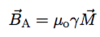
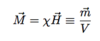
(Magnetization and Magnetic Susceptibility: 2 points)
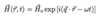
- External field leads to magnetization M
Macroscopic Quanities
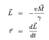
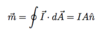
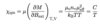
(Magnetic Moment: 2 points)
- Classically given as (see below)
- When current due to single electron, I = -e/T with T = 2πr /v
Macroscopic Quantities
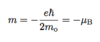
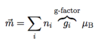
(Magnetic Moment [Bohr Magneton]: 2 points)
- Consider Bohn quantization of orbital momentum L = movr ≡ (\hbar) → Bohr magneton
Macroscopic Quantities
(Magnetic Moment [For Solid])
Macroscopic Quantities
(Magnetic Permeability)

Macroscopic Quantities
(Local Magnetic Field Hloc: 4 points)
- Similar as for local electric field
- Demagnetization field HN = -NM
- Lorentz field HL = M /3
- HL very small in para-/diamagnetic material because χ << 1
Macroscopic Quantities
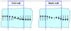
(Demagnetization and Stray Field [Consider]: 2 points)
- Thin disk of ferromagnetic material
- Homogenous mangetization along normal of disk N = 1
Macroscopic Quantities
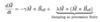
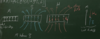
(Demagnetization and Stray Field [Take-Away]: 4 points and diagram)
- M induces B
- Inside disk: demagnetization field HN = B /µo - M
- Outside disk: stray field Hs = B /µo
- Amperes law only holds if Hs and HN in opposite directions
Macroscopic Quantity
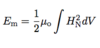
(Magnetostatic Self-Energy: 4 points)
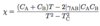
- Magnetostatic self-energy Em arises between each atomic magnetic moment interacts with the magnetic field create by all other moments in solid
- Energy of one magnetic moment µ in Hloc is Eµ = -µoµHloc
- Integrate over entire volume to get total self-energy (see below)
Microscopic Theory of Magnetic Properties
(Diamagnetic Solids: 2 points)
- Hext = 0 → no magnetic moments
- Hext > 0 → finite magnetization from induced magnetic moment opposite to applied field M = χdiH for χdi < 0
Microscopic Theory of Magnetic Properties
(Diamagnetic Solids [Types]: 6 points)
- Two types
-
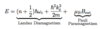
Larmor Diamagnetism:
- atomic diamagnetism in insulator
- magnetic moments due to atoms or tightly bound electrons
-
Landau Diamagnetism:
- Magnetization of free electrons in metals
-
Larmor Diamagnetism:
Microscopic Theory of Magnetic Properties
(Paramagnetic Solids: 3 points)
- Magnetic moments even for Hext = 0
- Due to orbital electron motion µL or spin of crystal electrons µS
- Hext > 0 → magnetic moments align with external field M = χpaH with χpa > 0
Microscopic Theory of Magnetic Properties
(Russel-Saunders Coupling: 2 points)
- Orbital momenta couple to total orbital momenum L = ∑ili and spin couple to total spin S = ∑isi
- Total angular momentum given by Russel-Saunders Coupling J = L + S
Microscopic Theory of Magnetic Properties
(Paramagnetic Solids [Types]: 4 points)
-
Langevin Paramagnetism:
- due to atomic paramagnetism in insulators
-
Pauli Paramagnetism:
- due to conducting electrons in metals
Microscopic Theory of Magnetic Properties
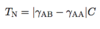
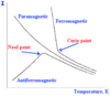
(Ferromagnetic Materials: 5 points)
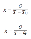
- For T < Tc → spontaneous magnetization without external field
- Results from exchange interaction causing spatial ordering of permanent magnetic moments
- Exchange interactions purely quantum mechanical:
- Pauli Principle
- Coulomb interaction
Microscopic Theory of Magnetic Properties
(Langevin Paramagnetism: 4 points)
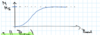
- Classical description (good for large J)
- Look at thermodynamic value of magnetization M = nV<µz>
- For high Bext → <µz> = µ
- Saturation magnetization Ms = nVµ
Microscopic Theory of Magnetic Properties
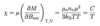
(Langevin Paramagnetism [Curie Law])
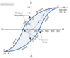
Microscopic Theory of Magnetic Properties
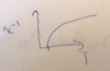
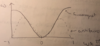
(Langevin Paramagnetism: diagram)
Microscopic Theory of Magnetic Properties
(Langevin Paramagnetism [QM Curie Law]: 2 points)
- two-level system
- similar description as classical Cure Law (up to factor 1/3)
Para-/Diamagnetism of Metal
(Overview: 3 points)
- Recall: Effect of B-field on free electrons → Landau Diamagnetism
- Add contribution from electron spin → Pauli Paramagnetism
Para-/Diamagnetism of Metal
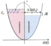
(Pauli Paramagnetism [Overview]: 2 points)
- Electron spin magnetic µs moment can take two values µs = ±µB
- Magnetization M = (n+ − n-)µB is function of spin-up/-down densities
Para-/Diamagnetism of Metal
(Pauli Paramagnetism [Curie Law]: 6 points)
-
Expectation:
- Curie-Law M = C /T
-
Reality:
- Curie Constant is no longer constant C = C(T)
-
Explanation:
- Only electrons near EF can respond to field, and this population increases with T