Starting

Question 1

Conversation laws

Answer 1

We consider a quantity Q that varies in space, ~x, and time, t, with density u(~x, t),
flux ~q (~x, t), and source density σ (~x, t).
For example, if Q is the mass of a chemical species diffusing through a stationary
medium, we may take u to be the density, ~q the mass flux, and f the mass rate per
unit volume at which the species is generated.
For simplicity, we suppose that u(x, t) is scalar-valued, but exactly the same
considerations would apply to a vector-valued density (leading to a system of equations).

Question 2

Constitutive equations

Answer 2

The conservation law (1.2) is not a closed equation for the density u. Typically,
we supplement it with constitutive equations that relate the flux ~q and the source
density σ to u and its derivatives. While the conservation law expresses a general physical principle, constitutive equations describe the response of a particular
system being modeled

Question 3

KPP equation( we discuss a specific example of an equation that arises as a model 
in population dynamics and genetics)

Answer 3

3. 1. Reaction-diffusion equations
4. 2. Maximum principle
5. 3. Logistic equation
6. 4. Nondimensionalization
7. 5. Traveling waves
8. 6. The existence of traveling waves
9. 7. The initial value problem

Question 4

3.1. Reaction-diffusion equations

Answer 4

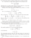
If ~q = −ν∇u and σ = f(u) in (1.2), we get a reaction-diffusion equation
ut = ν∆u + f(u).
Spatially uniform solutions satisfy the ODE
ut = f(u),
which is the ‘reaction’ equation. In addition, diffusion couples together the solution
at different points.

Question 5

3.2. Maximum principle

Answer 5

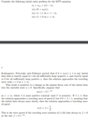
According to the maximum principle, the solution of (1.5) remains nonnegative if
the initial data u0(x) = u(x, 0) is non-negative, which is consistent with its use as
a model of population or probability.
The maximum principle holds because if u first crosses from positive to negative
values at time t0 at the point x0, and if u(x, t) has a nondegenerate minimum at x0,
then uxx(x0, t0) > 0. Hence, from (1.5), ut(x0, t0) > 0, so u cannot evolve forward
in time into the region u < 0. A more careful argument is required to deal with
degenerate minima, and with boundaries, but the conclusion is the same [18, 42]

Question 6

3.3. Logistic equation

Answer 6

Spatially uniform solutions of (1.5) satisfy the logistic equation
(1.6) ut = ku(a − u).
This ODE has two equilibrium solutions at u = 0, u = a.
The solution u = 0 corresponds to a complete absence of the species, and
is unstable. Small disturbances grow initially like u0e
kat. The solution u = a
corresponds to the maximum population that can be sustained by the available
resources. It is globally asymptotically stable, meaning that any solution of (1.6)
with a strictly positive initial value approaches a as t → ∞.
Thus, the PDE (1.5) describes the evolution of a population that satisfies logistic dynamics at each point of space coupled with dispersal into regions of lower
population.

Question 7

Nondimensionalization

Answer 7

Question 8

3.5. Traveling waves

Answer 8

Question 9

3.6. The existence of traveling waves

Answer 9

Question 10

3.7. The initial value problem

Answer 10