Reading 11 - Sampling and Estimation

Question 1

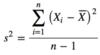
Sampling

Answer 1

In a simple random sample, each member of the population has the same probability
or likelihood of being included in the sample. For example, assume that our population consists of 10 balls labeled with numbers 1 to 10. Drawing a random sample of 3 balls from this population of 10 balls would require that each ball has an equal chance of being chosen in the sample, and each combination of balls has an identical chance of being the chosen sample as any other combination.

Question 2

Systematic sampling

Answer 2

In practice, random samples are generated using random number tables or computer random‐number generators. Systematic sampling is often used to generate approximately random samples. In systematic sampling, every kth member in the population list is selected until the desired sample size is reached.

Question 3

Systematic sampling

Answer 3

In practice, random samples are generated using random number tables or computer random‐number generators. Systematic sampling is often used to generate approximately random samples. In systematic sampling, every kth member in the population list is selected until the desired sample size is reached.

Question 4

Sampling error

Answer 4

Sampling error is the error caused by observing a sample instead of the entire population to draw conclusions relating to population parameters. It equals the difference between
a sample statistic and the corresponding population parameter.

Question 5

Sampling error of the mean

Answer 5

Sampling error of the mean = Sample mean − Population mean = x − μ

Question 6

Sampling distribution & sampling distribution of the mean

Answer 6

A sampling distribution is the probability distribution of a given sample statistic under repeated sampling of the population. Suppose that a random sample of 50 stocks is selected from a population of 10,000 stocks, and the average return on the 50‐stock sample is calculated. If this process were repeated several times with samples of the same size (50), the sample mean (estimate of the population mean) calculated will be different each time due to the different individual stocks making up each sample. The distribution of these sample means is called the sampling distribution of the mean.

Remember that all the samples drawn from the population must be random, and of the same size. Also note that the sampling distribution is different from the distribution of returns of each of the components of the population (each of the 10,000 stocks) and has different parameters.

Question 7

Stratification

Answer 7

Stratification is the process of grouping members of the population into relatively homogeneous subgroups, or strata, before drawing samples. The strata should be mutually exclusive i.e., each member of the population must be assigned to only one stratum. The strata should also be collectively exhaustive i.e., no population element should be excluded from the sampling process. Once this is accomplished, random sampling is applied within each stratum and the number of observations drawn from each stratum is based on the size of the stratum relative to the population. This often improves the representativeness of the sample by reducing sampling error.

Question 8

Time-series data

Answer 8

• ‐series data consists of observations measured over a period of time, spaced at uniform intervals. The monthly returns on a particular stock over the last 5 years are an example of time‐series data. 


Question 9

Cross-sectional data

Answer 9

Cross‐sectional data refers to data collected by observing many subjects (such as individuals, firms, or countries/regions) at the same point in time. Analysis of cross‐sectional data usually consists of comparing the differences among the subjects. The returns of individual stocks over the last year are an example of cross‐sectional data. 


Question 10

Data sets can have both time‐series and cross‐sectional data in them. Examples of such data sets are:

Answer 10

Longitudinal data, which is data collected over time about multiple characteristics of the same observational unit. The various economic indicators—unemployment levels, inflation, GDP growth rates (multiple characteristics) of a particular country (observational unit) over a decade (period of time) are examples of longitudinal data. 


Panel data, which refers to data collected over time about a single characteristic of multiple observational units. The unemployment rate (single characteristic) of a number of countries (multiple observational units) over time are examples of panel data.

Question 11

Central limit theorem

Answer 11

The central limit theorem allows us to make accurate statements about the population mean and variance using the sample mean and variance regardless of the distribution of the population, as long as the sample size is adequate. An adequate sample size is defined as one that has more than 30 observations (n ≥ 30). 


Question 12

The important properties of the central limit theorem are: 


Answer 12

1) Given a population with any probability distribution, with mean, μ, and variance, σ2, the sampling distribution of the sample mean x-bar, computed from sample size, n, will approximately be normal with mean, μ (the population mean), and variance, σ2/ n (population variance divided by sample size), when the sample size is greater than or equal to 30.
2) No matter what the distribution of the population, for a sample whose size is greater than or equal to 30, the sample mean will be normally distributed. 


x̅ ~ N(μ,( σ²/n))

3) The mean of the population (μ) and the mean of the distribution of sample means x are equal. 

4) The variance of the distribution of sample means equals σ²/n, or population variance divided by sample size.

Question 13

Standard error

Answer 13

The standard deviation of the distribution of sample means is known as the standard error of the statistic. 


Question 14

When the population variance, σ 2, is known, the standard error of sample mean is calculated as: 


Answer 14

Question 15

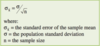
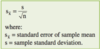
Practically speaking, population variances are almost never known, so we estimate the standard error of the sample mean using the sample’s standard deviation:

Answer 15

Question 16

Point estimate

Answer 16

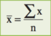
A point estimate involves the use of sample data to calculate a single value (a statistic) that serves as an approximation for an unknown population parameter. For example, the sample mean, x, is a point estimate of the population mean, μ. The formula used to calculate a point estimate is known as an estimator.

Question 17

The estimator for the sample mean is given as:

Answer 17

Question 18

Confidence interval

Answer 18

A confidence interval uses sample data to calculate a range of possible (or probable) values that an unknown population parameter can take, with a given of probability of
(1 – α). α is called the level of significance, and (1 – α) refers to the degree of confidence that the relevant parameter will lie in the computed interval. For example, a calculated interval between 100 and 150 at the 5% significance level implies that we can be 95% confident that the population parameter will lie between 100 and 150.

Question 19

A (1 – α)% confidence interval has the following structure:

Answer 19

Point estimate ± (reliability factor * standard error)

where:


Point estimate = value of the sample statistic that is used to estimate the population parameter.

Reliability factor = a number based on the assumed distribution of the point estimate and the level of confidence for the interval (1 – α).

Standard error = the standard error of the sample statistic (point estimate).

Question 20

When choosing between a number of possible estimators for a particular population parameter, we make use of the desirable statistical properties of an estimator to make the best possible selection. The desirable properties of an estimator are:

Answer 20

Unbiasedness

Efficiency

Consistency

Question 21

Statistical property: Unbiasedness

Answer 21

Unbiasedness: An unbiased estimator is one whose expected value is equal to the parameter being estimated. The expected value of the sample mean equals the population mean [E(x) = μ]. Therefore, the sample mean, x, is an unbiased estimator of the population mean, μ . 


Question 22

Statistical property: Efficiency

Answer 22

Efficiency: An efficient unbiased estimator is the one that has the lowest variance among all unbiased estimators of the same parameter. 


Question 23

Statistical property: Consistency

Answer 23

Consistency: A consistent estimator is one for which the probability of estimates close to the value of the population parameter increases as sample size increases. We have already seen that the standard error of the sampling distribution falls as sample size increases, which implies a higher probability of estimates close to the population mean.

Question 24

Student’s t‐distribution is a bell‐shaped probability distribution that has the following properties:

Answer 24

• It is symmetrical. 

• It is defined by a single parameter, the degrees of freedom (df), where degrees of 
freedom equal sample size minus one (n‐1). 

• It has a lower peak than the normal curve, but fatter tails. 

• As the degrees of freedom increase, the shape of the t‐distribution approaches the 
shape of the standard normal curve. 


Question 25

A random sample size, n, and degrees of freedom

Answer 25

A random sample of size, n, is said to have n‐1 degrees of freedom. Basically, there are n‐1 independent deviations from the mean on which the estimate can be based.

Question 26

What happens to the t-distribution curve as degrees of freedom increase?

Answer 26

As the degrees of freedom increase, the t‐distribution curve becomes more peaked
and its tails become thinner (bringing it closer to a normal curve). As a result, for a
given significance level, the confidence interval for a random variable that follows the t‐distribution will become narrower when the degrees of freedom increase. We will be more confident that the population mean will lie within the calculated interval as more data is concentrated towards the middle (as demonstrated by the higher peak) and less data is in the tails (thinner tails). 


Question 27

The t‐distribution is used in the following scenarios:

Answer 27

• It is used to construct confidence intervals for a normally (or approximately normally) distributed population whose variance is unknown when the sample size is small (n < 30). 

• It may also be used for a non‐normally distributed population whose variance is unknown if the sample size is large (n ≥ 30). In this case, the central limit theorem is used to assume that the sampling distribution of the sample mean is approximately normal. 


Question 28

The confidence interval for the population mean when the population follows a normal distribution and its variance is known is calculated as follows: 
(NOTE: works if you have population standard deviation)

Answer 28

Question 29

The following reliability factors are used frequently when constructing confidence intervals based on the standard normal distribution:

Answer 29

For a 90% confidence interval we use z0.05 = 1.65 


For a 95% confidence interval we use z0.025 = 1.96 


For a 99% confidence interval we use z0.005 = 2.58 


Question 30

This confidence interval can be interpreted in two ways:

Answer 30

• Probabilistic interpretation*: After repeatedly taking samples of 36 SAT candidates’ scores on the mock exam, and then constructing confidence intervals based on each sample’s mean, 99% of the confidence intervals will include the population mean over the long run. 

• Practical interpretation*: We can be 99% confident that the average population score for the actual SAT exam is between 1663 and 1836. 


Question 31

When the variance of a normally distributed population is not known, we use the t‐distribution to construct confidence intervals:

Answer 31

Question 32

t-distribution vs. z-distribution

Answer 32

Recall that the critical t‐values or the reliability factor for constructing the confidence interval depends on the level of confidence desired, and on the sample size. Also recall that the t‐distribution has fatter or thicker tails relative to the normal distribution. Since more observations essentially lie in the tails of the distribution, a confidence interval for a given significance level will be broader for the t‐distribution compared to the z‐distribution.

Question 33

When the population is normally distributed, when do we use z-statistic vs t-statistic?

Answer 33

Use the z‐statistic when the population variance is known. 


Use the t‐statistic when the population variance is not known.



Question 34

When the distribution of the population is nonnormal, the construction of an appropriate 
confidence interval depends on the size of the sample. 
When do we use z-statistic vs t-statistic?

Answer 34

• If the population variance is known and the sample size is large (n ≥ 30) we use the z‐statistic. This is because the central limit theorem tells us that the distribution of the sample mean is approximately normal when sample size is large. 

• If the population variance is not known and sample size is large, we can use the z‐statistic or the t‐statistic. However, in this scenario the use of the t‐statistic is encouraged because it results in a more conservative measure. 


This implies that we cannot construct confidence intervals for nonnormal distributions if sample size is less than 30. 


Question 35

When do you use z-distribution to construct confidence intervals?

Answer 35

When the variance of a normally distributed population is not known, and the sample size is large we use the z‐distribution to construct confidence intervals: 


Question 36

Criteria for Selecting Appropriate Test Statistic

Answer 36

Question 37

From our discussion so far, we have understood that there are various factors that affect the width of a confidence interval: Name two.

Answer 37

The choice of test statistic: A t‐statistic gives a wider confidence interval. 


The degree of confidence: A higher desired level of confidence increases the size 
of the confidence interval. 


Question 38

From our formula for the confidence interval, it is easy to see that the width of the interval is also a function of the standard error. 
Explain.

Answer 38

The larger the standard error, the wider the confidence interval. The standard error, in turn, is a function of sample size. More specifically, a larger sample size results in a smaller standard error and reduces the width of the confidence interval. Therefore, large sample sizes are desirable as they increase the precision with which we can estimate a population parameter. However, in practice two considerations may work against increasing the sample size: 


Increasing the size of the sample may result in drawing observations from a different population. 


Increasing the sample size may involve additional expenses that outweigh the benefit of increased accuracy of estimates. 
Other than the risk of sampling from more than one population, there are a variety of challenges to valid sampling. If the sample is biased in any way, estimates and conclusions drawn from sample data will be erroneous. 


Question 39

Name the types of biases

Answer 39

Data mining bias

Sample selection bias

Survivorship bias

Look-ahead bias

Time-period bias

Question 40

Data mining

Answer 40

Data mining is the practice of developing a model by extensively searching through a data set for statistically significant relationships until a pattern “that works” is discovered. In the process of data mining, large numbers of hypotheses about a single data set are tested in a very short time by searching for combinations of variables that might show a correlation. 


Given that enough hypotheses are tested, it is virtually certain that some of them will appear to be highly statistically significant, even on a data set with no real correlations at all. Researchers who use data mining techniques can be easily misled by these apparently significant results even though they are merely coincidences. 


Question 41

Data‐mining bias most commonly occurs when:

Answer 41

Researchers have not formed a hypothesis in advance, and are therefore open to 
any hypothesis suggested by the data. 


When researchers narrow the data used in order to reduce the probability of the 
sample refuting a specific hypothesis. 


Question 42

Warning signs that data mining bias might exist are:

Answer 42

• Too much digging warning sign*, which involves testing numerous variables until one that appears to be significant is discovered. 

• No story/ no future warning sign*, which is indicated by a lack of an economic theory that can explain empirical results. 


Question 43

The best way to avoid the data‐mining bias is to:

Answer 43

The best way to avoid the data‐mining bias is to test the “apparently statistically significant relationships” on “out‐of‐sample” data to check whether they continue to hold. 


Question 44

Sample-selection bias

Answer 44

Sample-selection bias results from the exclusion of certain assets (such as bonds, stocks, or portfolios) from a study due to the unavailability of data. 


Sample selection bias is even more severe in studies of hedge fund returns. This is because hedge funds are not required to publicly disclose their performance data. Only funds that performed well choose to disclose their performance, which leads to an overstatement of hedge fund returns. 


Question 45

Survivorship bias

Answer 45

Some databases use historical information and may suffer from a type of sample selection bias known as survivorship bias. This bias is present in databases that only list companies or funds currently in existence, which means that those that have failed are not included in the database. As a result, the results obtained from the study may not accurately reflect the true picture. 


Question 46

Look-Ahead Bias

Answer 46

Look‐ahead bias arises when a study uses information that was not available on the test date. For example, consider a test on a trading rule based on the price‐to‐book value ratio of stocks. Stock prices are usually easily available, but year-end book values are not available till the first quarter of the next year (when financial statements are released). 


Question 47

Time-Period Bias

Answer 47

Time‐period bias arises if a test is based on a certain time period, which may make the results obtained from the study time‐period specific. If the selected time period is relatively short, results will reflect relationships that held only during that particular period. On the other hand, if the time period is too long, the study might fail to uncover any structural changes that occurred during the period. 


Question 48

Reading 11 – Sampling and estimation – Learning outcomes

Answer 48

The candidate should be able to:

• define simple random sampling and a sampling distribution;
• explain sampling error;
• distinguish between simple random and stratified random sampling;
• distinguish between time-series and cross-sectional data;
• explain the central limit theorem and its importance;
• calculate and interpret the standard error of the sample mean;
• identify and describe desirable properties of an estimator;
• distinguish between a point estimate and a confidence interval estimate of a population parameter;
• describe properties of Student’s t-distribution and calculate and interpret its degrees of freedom;
• calculate and interpret a confidence interval for a population mean, given a normal distribution with 1) a known population variance, 2) an unknown population variance, or 3) an unknown variance and a large sample size;

- describe the issues regarding selection of the appropriate sample size, data-mining bias, sample selection bias, survivorship bias, look-ahead bias, and time-period bias.

Question 49

Sampling plan

Answer 49

The set of rules used to select a sample.

Question 50

Simple random sample

Answer 50

A subset of a larger population created in such a way that each element of the population has an equal probability of being selected to the subset.

Question 51

Systematic Sampling

Answer 51

A procedure of selecting every kth member until reaching a sample of the desired size. The sample that results from this procedure should be approximately random.

Question 52

Sampling error

Answer 52

The difference between the observed value of a statistic and the quantity it is intended to estimate.

Question 53

Sampling distribution

Answer 53

The distribution of all distinct possible values that a statistic can assume when computed from samples of the same size randomly drawn from the same population.

Question 54

Stratified Random Sampling

Answer 54

Definition of Stratified Random Sampling. In stratified random sampling, the population is divided into subpopulations (strata) based on one or more classification criteria. Simple random samples are then drawn from each stratum in sizes proportional to the relative size of each stratum in the population. These samples are then pooled to form a stratified random sample.

Question 55

Indexing

Answer 55

An investment strategy in which an investor constructs a portfolio to mirror the performance of a specified index.

Question 56

Pure bond indexing

Answer 56

Bond indexing is one area in which stratified sampling is frequently applied. Indexing is an investment strategy in which an investor constructs a portfolio to mirror the performance of a specified index. In pure bond indexing, also called the full-replication approach, the investor attempts to fully replicate an index by owning all the bonds in the index in proportion to their market value weights. Many bond indexes consist of thousands of issues, however, so pure bond indexing is difficult to implement. In addition, transaction costs would be high because many bonds do not have liquid markets.

Question 57

How does stratified random indexing help pure bond indexing

Answer 57

Because the major risk factors of fixed-income portfolios are well known and quantifiable, stratified sampling offers a more effective approach. In this approach, we divide the population of index bonds into groups of similar duration (interest rate sensitivity), cash flow distribution, sector, credit quality, and call exposure. We refer to each group as a stratum or cell (a term frequently used in this context).¹ Then, we choose a sample from each stratum proportional to the relative market weighting of the stratum in the index to be replicated.

Question 58

Monetary policy

Answer 58

Actions taken by a nation’s central bank to affect aggregate output and prices through changes in bank reserves, reserve requirements, or its target interest rate.

Question 59

Sharpe ratio

Answer 59

The average return in excess of the risk-free rate divided by the standard deviation of return; a measure of the average excess return earned per unit of standard deviation of return.

Question 60

The reader may also encounter two types of datasets that have both time-series and cross-sectional aspects:

Answer 60

Panel data consist of observations through time on a single characteristic of multiple observational units. For example, the annual inflation rate of the Eurozone countries over a five-year period would represent panel data.

Longitudinal data consist of observations on characteristic(s) of the same observational unit through time. Observations on a set of financial ratios for a single company over a 10-year period would be an example of longitudinal data. Both panel and longitudinal data may be represented by arrays (matrixes) in which successive rows represent the observations for successive time periods.

Question 61

The Central Limit Theorem

Answer 61

Given a population described by any probability distribution having mean μ and finite variance σ², the sampling distribution of the sample mean X-Bar computed from samples of size n from this population will be approximately normal with mean μ (the population mean) and variance σ²/n (the population variance divided by n) when the sample size n is large.

Question 62

The estimate of s is given by the square root of the sample variance, s², calculated as follows:

Answer 62

Question 63

Lower bound

Answer 63

The lowest possible value of an option.

Question 64

Random variables mean and variance equations

Answer 64

If a is the lower limit of a uniform random variable and b is the upper limit, then the random variable’s mean is given by (a + b)/2 and its variance is given by (b − a)²/12. The reading on common probability distributions fully describes continuous uniform random variables.

Question 65

To summarize, according to the central limit theorem, when we sample from any distribution, the distribution of the sample mean will have the following properties as long as our sample size is large:

Answer 65

- The distribution of the sample mean X-BAR


will be approximately normal.

• The mean of the distribution of X-BAR


will be equal to the mean of the population from which the samples are drawn.
• The variance of the distribution of X-BAR

will be equal to the variance of the population divided by the sample size.

Question 66

Estimator

Answer 66

An estimation formula; the formula used to compute the sample mean and other sample statistics are examples of estimators.

Question 67

Estimate

Answer 67

The particular value calculated from sample observations using an estimator.

Question 68

Point Estimate

Answer 68

A single numerical estimate of an unknown quantity, such as a population parameter.

Question 69

Definition of Unbiasedness

Answer 69

An unbiased estimator is one whose expected value (the mean of its sampling distribution) equals the parameter it is intended to estimate.

Question 70

Definition of Efficiency

Answer 70

An unbiased estimator is efficient if no other unbiased estimator of the same parameter has a sampling distribution with smaller variance.

Question 71

Definition of Consistency

Answer 71

A consistent estimator is one for which the probability of estimates close to the value of the population parameter increases as sample size increases.

Question 72

Confidence Interval

Answer 72

A confidence interval is a range for which one can assert with a given probability 1 − α, called the degree of confidence, that it will contain the parameter it is intended to estimate. This interval is often referred to as the 100(1 − α)% confidence interval for the parameter.

Question 73

Degree of confidence

Answer 73

The probability that a confidence interval includes the unknown population parameter.

Question 74

It is also possible to define two types of one-sided confidence intervals for a population parameter. Explain.

Answer 74

A lower one-sided confidence interval establishes a lower limit only. Associated with such an interval is an assertion that with a specified degree of confidence the population parameter equals or exceeds the lower limit. An upper one-sided confidence interval establishes an upper limit only; the related assertion is that the population parameter is less than or equal to that upper limit, with a specified degree of confidence. Investment researchers rarely present one-sided confidence intervals, however.

Question 75

Construction of Confidence Intervals

Answer 75

A 100(1 − α)% confidence interval for a parameter has the following structure. 


Point estimate ± Reliability factor × Standard error 

where

Point estimate = a point estimate of the parameter (a value of a sample statistic)

Reliability factor = a number based on the assumed distribution of the point estimate and the degree of confidence (1 − α) for the confidence interval

Standard error = the standard error of the sample statistic providing the point estimate

Question 76

Degrees of freedom (df)

Answer 76

The number of independent observations used.

Question 77

Basis of Computing Reliability Factors: Normal distribution with known variance

Answer 77

Statistic for small sample size: z

Statistic for large sample size: z

Question 78

Basis of Computing Reliability Factors: Normal distribution with unknown variance

Answer 78

Statistic for small sample size: t

Statistic for large sample size: t (or z)

Question 79

Basis of Computing Reliability Factors: Nonnormal distribution with known variance

Answer 79

Statistic for small sample size: Not available

Statistic for large sample size: z

Question 80

Basis of Computing Reliability Factors: Nonnormal distribution with unknown variance

Answer 80

Statistic for small sample size: Not available

Statistic for large sample size: t (or z)

Question 81

Data mining

Answer 81

The practice of determining a model by extensive searching through a dataset for statistically significant patterns. Also called data snooping.

Question 82

Out-of-sample test

Answer 82

A test of a strategy or model using a sample outside the time period on which the strategy or model was developed.

Question 83

Intergenerational data mining

Answer 83

A form of data mining that applies information developed by previous researchers using a dataset to guide current research using the same or a related dataset.

Question 84

McQueen and Thorley presented two signs that can warn analysts about the potential existence of data mining:

Answer 84

Too much digging/too little confidence

No story/no future

Question 85

McQueen and Thorley presented two signs that can warn analysts about the potential existence of data mining: Too much digging/ too little confidence.

Answer 85

Too much digging/too little confidence. The testing of many variables by the researcher is the “too much digging” warning sign of a data-mining problem. Unfortunately, many researchers do not disclose the number of variables examined in developing a model. Although the number of variables examined may not be reported, we should look closely for verbal hints that the researcher searched over many variables. The use of terms such as “we noticed (or noted) that” or “someone noticed (or noted) that,” with respect to a pattern in a dataset, should raise suspicions that the researchers were trying out variables based on their own or others’ observations of the data.

Question 86

McQueen and Thorley presented two signs that can warn analysts about the potential existence of data mining: No story/no future.

Answer 86

No story/no future. The absence of an explicit economic rationale for a variable or trading strategy is the “no story” warning sign of a data-mining problem. Without a plausible economic rationale or story for why a variable should work, the variable is unlikely to have predictive power. In a demonstration exercise using an extensive search of variables in an international financial database, Leinweber (1997) found that butter production in a particular country remote from the United States explained 75 percent of the variation in US stock returns as represented by the S&P 500. Such a pattern, with no plausible economic rationale, is highly likely to be a random pattern particular to a specific time period.²⁶ What if we do have a plausible economic explanation for a significant variable? McQueen and Thorley caution that a plausible economic rationale is a necessary but not a sufficient condition for a trading strategy to have value. As we mentioned earlier, if the strategy is publicized, market prices may adjust to reflect the new information as traders seek to exploit it; as a result, the strategy may no longer work.

Question 87

Sample selection bias

Answer 87

Bias introduced by systematically excluding some members of the population according to a particular attribute—for example, the bias introduced when data availability leads to certain observations being excluded from the analysis.

Question 88

Survivorship bias

Answer 88

The bias resulting from a test design that fails to account for companies that have gone bankrupt, merged, or are otherwise no longer reported in a database.

Question 89

Look-ahead bias

Answer 89

A bias caused by using information that was unavailable on the test date.

Question 90

Time-period bias

Answer 90

The possibility that when we use a time-series sample, our statistical conclusion may be sensitive to the starting and ending dates of the sample.

Question 91

How do you draw a valid inference from a sample?

Answer 91

To draw valid inferences from a sample, the sample should be random.

Question 92

How observations selected in simple random sampling & stratified random sampling?

Answer 92

In simple random sampling, each observation has an equal chance of being selected. In stratified random sampling, the population is divided into subpopulations, called strata or cells, based on one or more classification criteria; simple random samples are then drawn from each stratum.

Question 93

Why is stratified random sampling better than simple random sampling?

Answer 93

Stratified random sampling ensures that population subdivisions of interest are represented in the sample. Stratified random sampling also produces more-precise parameter estimates than simple random sampling.

Question 94

Time-series data vs. Cross-sectional data

Answer 94

Time-series data are a collection of observations at equally spaced intervals of time. Cross-sectional data are observations that represent individuals, groups, geographical regions, or companies at a single point in time.

Question 95

Central limit theorem

Answer 95

The central limit theorem states that for large sample sizes, for any underlying distribution for a random variable, the sampling distribution of the sample mean for that variable will be approximately normal, with mean equal to the population mean for that random variable and variance equal to the population variance of the variable divided by sample size.

Question 96

Based on the central limit theorem, when the sample size is large, what can we do?

Answer 96

Based on the central limit theorem, when the sample size is large, we can compute confidence intervals for the population mean based on the normal distribution regardless of the distribution of the underlying population. In general, a sample size of 30 or larger can be considered large.

Question 97

Estimator

Answer 97

An estimator is a formula for estimating a parameter. An estimate is a particular value that we calculate from a sample by using an estimator.

Question 98

Because an estimator or statistic is a random variable, how can it be described?

Answer 98

Because an estimator or statistic is a random variable, it is described by some probability distribution. We refer to the distribution of an estimator as its sampling distribution. The standard deviation of the sampling distribution of the sample mean is called the standard error of the sample mean.

Question 99

What are the desirable properties of an estimator?

Answer 99

The desirable properties of an estimator are unbiasedness (the expected value of the estimator equals the population parameter), efficiency (the estimator has the smallest variance), and consistency (the probability of accurate estimates increases as sample size increases).

Question 100

What are the two types of estimates of a parameter?

Answer 100

The two types of estimates of a parameter are point estimates and interval estimates. A point estimate is a single number that we use to estimate a parameter. An interval estimate is a range of values that brackets the population parameter with some probability.

Question 101

Confidence interval

Answer 101

A confidence interval is an interval for which we can assert with a given probability 1 − α, called the degree of confidence, that it will contain the parameter it is intended to estimate. This measure is often referred to as the 100(1 − α)% confidence interval for the parameter.

A 100(1 − α)% confidence interval for a parameter has the following structure: Point estimate ± Reliability factor × Standard error, where the reliability factor is a number based on the assumed distribution of the point estimate and the degree of confidence (1 − α) for the confidence interval and where standard error is the standard error of the sample statistic providing the point estimate.

Question 102

A 100(1 − α)% confidence interval for population mean μ when sampling from a normal distribution with known variance σ²is given by:

Answer 102

A 100(1 − α)% confidence interval for population mean μ when sampling from a normal distribution with known variance σ2 is given by x̅ ± zα/2*(σ/√n), where zα/2 is the point of the standard normal distribution such that α/2 remains in the right tail

Question 103

Student’s t-distribution

Answer 103

Student’s t-distribution is a family of symmetrical distributions defined by a single parameter, degrees of freedom.

Question 104

Degrees of freedom

Answer 104

A random sample of size n is said to have n − 1 degrees of freedom for estimating the population variance, in the sense that there are only n − 1 independent deviations from the mean on which to base the estimate.

Question 105

The degrees of freedom number for use with the t-distribution

Answer 105

The degrees of freedom number for use with the t-distribution is also n − 1.

Question 106

t-distribution description

Answer 106

The t-distribution has fatter tails than the standard normal distribution but converges to the standard normal distribution as degrees of freedom go to infinity.

Question 107

Compare the standard normal distribution and Student’s t-distribution

Answer 107

Basically, only one standard normal distribution exists, but many t-distributions exist—one for every different number of degrees of freedom. The normal distribution and the t-distribution for a large number of degrees of freedom are practically the same. The lower the degrees of freedom, the flatter the t-distribution becomes. The t-distribution has less mass (lower probabilities) in the center of the distribution and more mass (higher probabilities) out in both tails. Therefore, the confidence intervals based on t-values will be wider than those based on the normal distribution. Stated differently, the probability of being within a given number of standard deviations (such as within ±1 standard deviation or ±2 standard deviations) is lower for the t-distribution than for the normal distribution.

Question 108

A 100(1 − α)% confidence interval for the population mean μ when sampling from a normal distribution with unknown variance (a t-distribution confidence interval) is given by:

Answer 108

A 100(1 − α)% confidence interval for the population mean μ when sampling from a normal distribution with unknown variance (a t-distribution confidence interval) is given by x̅ ± t_α/2*(s/√n), where t_α/2 is the point of the t-distribution such that α/2 remains in the right tail and s is the sample standard deviation. This confidence interval can also be used, because of the central limit theorem, when dealing with a large sample from a population with unknown variance that may not be normal.

Question 109

We may use the confidence interval _____ as an alternative to the t-distribution confidence interval for the population mean when using a large sample from a population with unknown variance.

Answer 109

We may use the confidence interval x̅ ± z_α/2*(s/√n) as an alternative to the t-distribution confidence interval for the population mean when using a large sample from a population with unknown variance. The confidence interval based on the z-statistic is less conservative (narrower) than the corresponding confidence interval based on a t-distribution.

Question 110

Three issues in the selection of sample size

Answer 110

Three issues in the selection of sample size are the need for precision, the risk of sampling from more than one population, and the expenses of different sample sizes.

Question 111

Sample data in investments can have a variety of problems. Name and describe the biases.

Answer 111

Sample data in investments can have a variety of problems. Survivorship bias occurs if companies are excluded from the analysis because they have gone out of business or because of reasons related to poor performance. Data-mining bias comes from finding models by repeatedly searching through databases for patterns. Look-ahead bias exists if the model uses data not available to market participants at the time the market participants act in the model. Finally, time-period bias is present if the time period used makes the results time-period specific or if the time period used includes a point of structural change.