Quant Flashcards
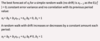
Calculate and interpret a sample covariance and a sample correlation coefficient (r).
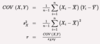
Identify the two sources of uncertainty when the regression model is used to make a prediction regarding the value of the dependent variable.
The uncertainty inherent in the error term, ε.
The uncertainty in the estimated parameters, b0 and b1.
Calculate and interpret a confidence interval for the predicted value of the dependent variable.
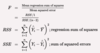
Explain the analysis of variance (ANOVA).
ANOVA describes the usefulness of the independent variables in capturing variation in the dependent variable.
RSS + SSE = Total variation. (Note that SSE is different from SEE.)
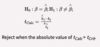
Formulate a null and alternative hypothesis about a population value of a regression coefficient and determine the appropriate test statistic and whether to reject the null hypothesis.
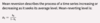
Calculate and interpret the F-stat.
Give the formula used to determine the linear regression model between the dependent and independent variables.
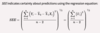
Calculate and interpret the standard error of the estimate (SEE).
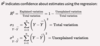
Calculate and interpret the coefficient of determination (R2).
List the five assumptions of the linear regression model.
Linearity within the parameters, b1 and b0.
The independent variable, X, is not random.
E(ε) = 0.
The variance of the error term is constant for all observations (i.e., homoskedasticity).
Uncorrelated, normally distributed errors.
Explain how time-series variables should be analyzed for nonstationarity and/or cointegration before use in a linear regression.
If the dependent variable or any independent variable has a unit root and at least one time series does not, multiple linear regression cannot be used due to nonstationarity.
If all of them have unit roots, the time series must be tested for cointegration as outlined previously.
Distinguish between unconditional and conditional heteroskedasticity.
Heteroskedasticity describes an inconsistent error term across observations.
Unconditional – Not related to independent variables in the regression; does not create major problems for statistical inference.
Conditional – Correlated with the independent variables in the regression; does create problems but can be identified and corrected.
Identify the two ways to correct for conditional heteroskedasticity in linear regression models.
Robust standard errors – Corrects standard errors for the conditional heteroskedasticity.
Generalized least squares – Modifies the regression equation for conditional heteroskedasticity. This requires econometrics expertise.
What are the two approaches to check for seasonality?
Graph the data and check for regular seasonal patterns.
Examine the data to see whether the seasonal autocorrelations of the residuals from an AR model are significant and whether other autocorrelations are significant.
Explain the two options when making an initial choice of model.
A regression model that predicts the future behavior of a variable based on hypothesized causal relationships with other variables.
A time-series model that attempts to predict the future behavior of a variable based on the past behavior of the same variable.
Describe the autoregressive moving-average (ARMA) models.
An ARMA (p,q) model combines autoregressive lags of the dependent variable (p) and moving-average errors (q) in order to provide better forecasts than simple AR models.
Why are moving averages generally calculated?
To focus on the underlying trend by eliminating “noise” from a time series.
Identify the two situations that must be met for an AR model to be estimated using ordinary least squares.
Calculate the predicted trend for a linear time series given the coefficients.
Describe factors that determine whether a linear or a log-linear trend should be used.
Explain mean reversion and calculate a mean-reverting level.
How is the Durbin-Watson (DW) test approximated?
Describe how model misspecification affects regression results.
Failing to transform variables can lead to increasing error terms that violate regression assumptions of homoskedasticity.
Omitting important variables can lead to biased and inconsistent estimations for the regression coefficients.
Explain how autocorrelation of residuals can be used to test whether a model fits the time series.
First, assume that the expected value for the error term in a time series model is 0. Perform a hypothesis test; if the absolute value of t-calc is higher than t-critical, accept the null hypothesis that the autocorrelation is not significantly different from 0.
Evaluate limitations of trend models
Describe characteristics of random walk processes.
Identify the steps to determine which autoregressive model to use.
Give scenarios where the F-test and individual t-tests on the slope coefficients may offer conflicting conclusions.
We may reject the null hypothesis that all the slope coefficients equal zero based on the F-test even though individual slope coefficient t-tests cannot reject the null hypothesis.
We may fail to reject the null hypothesis that all the slope coefficients equal zero based on the F-test even though individual slope coefficient t-tests reject the null hypothesis.
Explain dummy variables in regression models.
List the steps to use a linear trend or an exponential trend to model a time series.
Plot the series to determine whether a linear or exponential trend seems most reasonable.
Use the developed model for forecasting if the Durbin-Watson statistic indicates no significant serial correlation in the residuals.
Explain coefficient instability of time series models.
Calculate the predicted trend for a log-linear time series given the coefficients.
Contrast random walk processes with covariance stationary processes.
Explain an autoregressive (AR) model.
Define multicollinearity.
Multicollinearity occurs when two or more independent variables (or combinations of independent variables) in a regression model are highly correlated with each other.
Describe models used with qualitative dependent variables.
Qualitative dependent variables are dummy variables representing a state of being (e.g., bankrupt or not). The probit model estimates the probability of a qualitative condition using a normal distribution while the logit model uses the heavier-tailed and higher kurtosis logistic distribution.
Discriminant analysis uses a linear function like regression to create overall scores used to classify observations qualitatively.
Give the equation used to determine the multiple linear regression model.
Describe the effects of heteroskedasticity on regression reliability.
Heteroskedasticity can lead to false inferences about the independent variable but does not affect the consistency of estimators of regression parameters. Both the F-test and t-tests can become unreliable, the latter due to bias introduced into standard errors of the regression coefficients.
Explain how to test and correct for seasonality in a time-series model.
Describe the two ways to determine whether a time series is covariance stationary.
Examine for statistically significant autocorrelation for any residual.
Conduct the Dickey-Fuller test for unit root (preferred approach).
How is the out-of-sample forecasting performance of autoregressive models evaluated?
On the basis of their root mean square error (RMSE). The RMSE for each model under consideration is calculated based on out-of-sample data. The model with the lowest RMSE has the lowest forecast error and hence carries the most predictive power.
Explain how time-series autocorrelations can also be used to determine whether an autoregressive or a moving-average model is more appropriate to fit the data.
List the requirements for a time series to be covariance stationary and describe the significance of a series that is not stationary.
The mean, variance, and covariance of the series with itself in the past or future must be constant and finite. Otherwise, model output has no economic meaning.
Give the moving-average (MA) model of order 1 calculation.
Identify the possible scenarios regarding the outcome of the Dickey-Fuller tests with Eagle-Granger critical values on two time series.
Use linear regression when 1) neither series (dependent or independent variable) has a unit root or 2) both series have a unit root but are cointegrated (i.e., share a common trend and have bounded divergence over time).
Do not use linear regression if 1) either (but not both) series has a unit root or 2) both series have a unit root and are not cointegrated.
Explain how multicollinearity affects a regression’s explanatory power.
Identify the two ways to correct for serial correlation in the regression residuals.
Hansen’s method - Adjusts standard errors for the coefficients. The coefficients stay the same, but the standard errors change. Robust standard errors for positive correlation are then larger.
Modify the regression equation to eliminate the serial correlation.
List the limitations of ARMA models.
Unstable parameters.
No set criteria for determining p and q.
Poor forecasting ability.
Distinguish between positive and negative serial correlation.
How are autoregressive conditional heteroscedasticity (ARCH) models used?
ARCH models are used to determine whether the variance of the error in one period depends on the variance of the error in previous periods.
Describe the Breusch-Pagan (BP) test.
Describe objectives, methods, and examples of data exploration.
Data exploration is used to investigate and comprehend data distributions and relationships:
Exploratory data analysis (EDA) is the first step in data exploration.
Feature selection involves selecting only pertinent data for ML model training; fewer features create less complex models that require less time to train.
Feature engineering involves creating new features by changing or transforming existing ones.
Describe preparing, wrangling, and exploring text-based data for financial forecasting.
A corpus is any collection of raw text data, which can be organized into a table containing two columns: (sentence) is for text and (sentiment) is for the corresponding sentiment class. The separator character (@) splits the data into text and sentiment class columns
Describe overfitting and identify ways of addressing it.
Describe objectives, steps, and techniques in model training.
Step 1: Method selection
Dataset Size: Small datasets can lead to underfitting because they are not sufficient to expose patterns in the data.
Number of Features: A small/large number of features can lead to underfitting/overfitting.
Describe objectives, steps, and examples of preparing and wrangling data.
Structured: Wrangling >> Transforming and scaling data
Describe objectives, steps, and examples of preparing and wrangling data.
Structured: Handling outliers
Describe methods for extracting, selecting, and engineering features from textual data.
A cleansed and preprocessed dataset is partitioned using a common ratio of 60:20:20, respectively:
Training set (60%)
Cross-validation set (20%)
Test set (20%)
Describe objectives, steps, and techniques in model training.
Method selection: Splitting the master data set.
A training set should include approximately 60% of the master dataset.
A cross-validation set (CV set) to tune and validate the model should constitute approximately 20% of the master dataset.
A test set uses the remaining data, which are split using random sampling techniques; for unsupervised learning, splitting is not needed.
Describe objectives, steps, and examples of preparing and wrangling data.
Unstructured: Text cleansing
Remove html tags: Most text data from web pages have html markup tags.
Remove punctuations: Most punctuations are unnecessary, but some may be useful for ML training.
Remove numbers: If numbers are in the text, they should be removed or substituted with an annotation /number/.
Remove white spaces: White spaces should be identified and removed to keep the text intact and clean.
Distinguish between supervised and unsupervised machine learning.
Describe objectives, methods, and examples of data exploration.
Exploratory data analysis
Briefly describe supervised machine learning algorithms, including classification and regression trees, ensemble learning, and random forest classifiers.
State and explain the steps in a data analysis project.
Step 1: Conceptualization of the modeling task
Deciding on the output of the model (i.e., future price movements), how the model will be used, who will use it, and how it will be incorporated into the investment process.
State and explain the steps in a data analysis project.
Step 3: Data preparation and wrangling
Describe preparing, wrangling, and exploring text-based data for financial forecasting.
Describe objectives, steps, and techniques in model training.
The objective of model training is to minimize forecasting errors:
Method selection involves deciding which ML method(s) to use based on the classification task and type and size of data.
Performance evaluation uses complementary techniques to quantify and understand model performance.
Tuning seeks to improve model performance.
State and explain the steps in a data analysis project.
Step 4: Data exploration
Describe objectives, steps, and techniques in model training.
Step 3: Tuning
Two overall performance metrics are accuracy and F1 score; high scores suggest good performance.
Accuracy is the percentage of correctly predicted classes out of total predictions.
Accuracy = (TP + TN)/(TP + FP + TN + FN)
F1 score is the harmonic mean of precision and recall.
F1 score = (2 × P × R)/(P + R)
Describe objectives, steps, and examples of preparing and wrangling data.
Structured: Scaling
State and explain the steps in a data analysis project.
Step 5: Model training
Describe objectives, steps, and examples of preparing and wrangling data.
Cleansing data
Incompleteness error is when data are missing. Missing and not applicable/available values (NAs) must be omitted or replaced with “NA” and deleted or substituted with imputed values.
Invalidity error—data are outside of a meaningful range.
Inaccuracy error—data are not a measure of true value.
Inconsistency error—data conflict with other data points or reality.
Non-uniformity error—the data are not present in an identical format.
Duplication error—delete duplicate observations.
Describe preparing, wrangling, and exploring text-based data for financial forecasting.
Describe objectives, methods, and examples of data exploration.
Feature selection: Unstructured
Describe objectives, methods, and examples of data exploration.
Feature selection: Removing noisy features
Describe methods for extracting, selecting, and engineering features from textual data.
Describe objectives, steps, and techniques in model training.
Step 2: Performance evaluation
What are the sources of out-of-sample error?
Bias error refers to the extent to which the inferred relationship fits the training data. Algorithms with erroneous assumptions produce high bias from underfitting and high in-sample error, leading to poor predictive value.
Variance error reflects how much the model’s results change in response to new data from validation and test samples. Unstable models pick up noise and spurious relationships, resulting in overfitting and high out-of-sample error.
Base error, which arises from randomness in the data.
State and explain the steps in a data analysis project.
Step 2: Data collection
Briefly describe supervised machine learning algorithms, including classification and regression trees, ensemble learning, and random forest classifiers.
Describe objectives, methods, and examples of data exploration.
Feature engineering
Numbers are converted into a token such as “/number/.”
N-grams are discriminative multi-word patterns with their connection kept intact. For example, a bigram such as “stock market” treats the two adjacent words as one.
Name entity recognition (NER) algorithm analyzes individual tokens and their surrounding semantics to tag an object class to the token.
Parts of speech (POS) uses language structure and dictionaries to tag every token with a corresponding part of speech. Some common POS tags are nouns, verbs, adjectives, and proper nouns.