CT4 - Models & Mortality

Question 1

What is a G Test?

Answer 1

G-tests are likelihood-ratio or maximum likelihood statistical significance tests that are increasingly being used in situations where chi-squared tests were previously recommended.

The G test is undertaken in the same way as a chi-squared test, with the same degrees of freedom.

If Oi is the observed frequency in a cell, E is the expected frequency on the null hypothesis, and the sum is taken over all non-empty cells, G is calculated as:

Question 2

How is a Pearson Residual Calculated?

Answer 2

For the Binomial mortality model (and thus approximately for the Poisson model), the Pearson residual is given by:

Question 3

What are the GLM Link Functions for the following DBNs?

• normal
• exponential
• poisson
• binomial

Answer 3

Question 4

Forward Selection Procedure for Levels of Nested Generalised Linear Models (GLMs)

Answer 4

Let Di be the deviance of the ith level model, where D0 is the deviance of the null model (G score, chi-squared or other with approx chi-squared dbn).

In turn test (D_i - D_i+1) against required significance level (normally 5%) in a chi-squared test with d.f. = 1.

If change in deviance is significant (i.e. p-value < 0.05), then this supports moving to the next level of model.

Question 5

Define a Symmetric Simple Random Walk

Answer 5

(Used to model processes, such as the movement of stock market share prices)

A simple random walk operates on discrete time and has a discrete state space (i.e. set of all integers)

Question 6

Define a Compound Poisson Process

Answer 6

A compound Poisson process is a continuous-time (random) stochastic process with jumps.

A compound Poisson proces operates on continous time. It has a discrete or continous state space depending on whether Y_j are continuous or discrete.

Examples:

• Aggregate claims for an insurance portfolio (number of claims, each of potentially differing size)
• Total rainfall (number of drops, each of differing size)
• Total biomass (number of patches of organism, each patch of differing size)

Question 7

What are the 12 Key Steps of Modelling

Answer 7

1. Objectives: Develop a clear set of objectives to model the relevant system or process, define its scope. This includes reviewing regulatory guidance.

2. Plan and validate: Plan the model around the chosen objectives, ensuring that the model’s output can be validated i.e. checked to ensure it accurately reflects the anticipated output from the relevant system or process.
3. Data: Collect and analyse the necessary data for the model. This will include assigning appropriate values to the input parameters and justifying any assumptions made as part of the modelling process.
4. Capture the real world system: The initial model should be described so as to capture the main features of the real world system. The level of detail in the model can always be reduced at a later stage. Choose parameters
5. Expertise: Involve the experts on the relevant system or process. They will be able to feedbacks on the validity of the model before it is developed further. Discuss worst cases and probabilities.
6. Choose a computer program: Decide on whether the model should be built using a simulation package or a general purpose language.
7. Write the model: Write the computer program for the model.
8. De-bug the program. (e.g. test against particular scenarios)
9. Test the model output: Test the reasonableness of the output from the model. The experts on the relevant system or process should be involved at this stage.
10. Review and amend: Review and carefully consider the appropriateness of the model in light of making small changes to the input parameters.
    
    • e.g. test median outcomes against business plans
    • e.g. check probabilities assigned to worst case scenarios
11. Analyse output: Analyse the output from the model. Test sensitivity to small changes.
12. Document and communicate: Communicate and document the results and the model.

Question 8

What are the Benefits of Modelling?

Answer 8

• Compressed timeframe
  (e. g. for financial planning, real world figures unfold over a lifetime, need to test over a shorter period)
• Ability to incorporate randomness
  (in stochastic models)
• **Scenario testing **
  (Can combine parameters in realistic scenarios - e.g. relating to interest rate rises)
• Greater control over experimental conditions
• Cost control
  (upstream testing cheaper than assessment after implementation)

Question 9

What are the Limitations of Modelling?

Answer 9

• Time and cost
  complex models are expensive to create
• Multiple runs required
  for stochastic models, gives an indication of the dbn of outputs, but shows the impact of changes to inputs, rather than optimising outputs
• Validation and verification
  Complex models are hard to relate back to the real world in sanity checking
• Reliance on data input
  rubbish in, rubbish out
• Inappropriate use
  Scope and purpose of model must be understood by client to avoid misuse
• Limited scope
  models can’t cover all future eventualities, such as changes in legislation
• Difficulty intepreting outputs
  results usually useful only relative to other results, not in absolute real-world terms

Question 10

Continuous, Discrete and Mixed Type Processes

Answer 10

In a stochastic (random) process, a family of random variables X_t : t ∈ τ is disclosed over time, t

In a discrete process, τ = {0, 1, 2, … }
= Z (natural, or counting numbers)
e.g. number of claims made

In a continuous process, T = R (real numbers), or [0,∞]
e.g. stock price fluctuations

A counting process N_t, is the number of events by time period t, where N_t is a non-decreasing integer and N₀ = 0

An example of a mixed type process, including both continuous and discrete elements, is the market price of coupon-paying bonds - the bonds change price at specific times in response to coupons being paid, but also change continually due to market.

Question 11

What is the Markov Property?

Answer 11

A process with the Markov property will be one in which the future development of the process may be predicted on the basis of the current state of the system alone, without reference to it past history.

If a stochastic process Xt is defined on a state space S and time set t ≥ 0, the Markov property is expressed mathematically as:

Question 12

Prove the Chapman-Kolmogorov Equations for n-step transitions

Answer 12

The Chapman-Kolmogorov Equations provide a way of calculating n-step transition probabilities through matrix multiplication of single-step transitions. The proof is as follows:

Question 13

How do you Calculate the
n-Step probability using the Chapman Kolmogorov equations?

Answer 13

If α_j0 is the initial probability distribution,

Question 14

Conditions for a Stationary Distribution in a Markov Chain

Answer 14

In a Markov chain, the distribution of X_n may converge to a limit π, such that

P(X_n= j | X₀= i) → π_j

Regardless of the starting point - this is known as a stationary distribution

• π_j = Σπ_ip_ij *for all i ∈ S
• A Markov chain with a finite state space has at least one stationary probability distribution}
• An irreducible Markov chain with a finite state space has a unique stationary probability distribution

Question 15

Time Inhomogeneous / Homogeneous Markov Chains

Answer 15

A Markov chain is called time-homogeneous if transition probabilities do not depend on time.

Where they do depend on time (e.g. risk for drivers at a particular age, or at a particular length of time after qualifying), a Markov Chain is called time-inhomogeneous.

Question 16

Simple No Claims Discount (NCD) Model

Answer 16

No Claims Discount (NCD)

Policy holders start at 0% level

No claim in year moves up one level (or stays at top)

Claim in year moves down one level (or stays at bottom)

e.g:

Consider a no claims discount (NCD) model for car-insurance premiums. The insurance
company offers discounts of 0%, 30% and 60% of the full premium, determined by the following rules:

1. All new policyholders start at the 0% level.
2. If no claim is made during the current year the policyholder moves up one discount level, or remains at the 60% level.
3. If one or more claims are made the policyholder moves down one level, or remains at the 0% level.

Transition graph shown below:

Question 17

# Define Transition Intensities *q<sub>ii</sub>(t), q<sub>ij</sub>(t)*
 for Markov Jump Processes

Answer 17

Question 18

Define Kolmogorov’s Forwards Equation for Markov Jump Processes

Answer 18

Question 19

Define Kolmogorovs Backwards Equation for Markov Jump Processes

Answer 19

Question 20

Distribution of Holding Times (Markov Jump Process)

Answer 20

Poisson process characterised by unit upward jumps - hence path fully characterised by times between jumps.

Distribution of Holding Times is Exponential with Parameter λ, in case of Poisson, and μ, in case of non-Poisson Markov Process.

Question 21

Define Residual and Current Holding Times for Markov Jump Processes

Answer 21

Question 22

What is the Survival Model?

Answer 22

The survival model is a two state Markov chain, with a state space of S = { A, D } (alive / dead). There is single transition rate μ(t) - identified with the force of mortality at age t

Question 23

What is the Sickness-Death Model?

Answer 23

An extension of the survival model, with three states - healthy (H), sick (S) or dead (D). S = { H, S, D }

Question 24

What is the Long Term Sickness Model?

Answer 24

The so-called long term care model is a time-inhomogeneous model where the rate of transition out of state S (sickness) will depend on the current holding time in state S.

Question 25

What is the Marriage Model?

Answer 25

The marriage model is a time-inhomogeneous model under which an individual can be either never married (B), married (M), divorced (D), widowed (W) or dead Δ. A Markov jump process can be formulated on the state space

S = { B, M, D, W, Δ }

Question 26

_{<span>Terminology for Model of Lifetime or Failure</span>}

Define: T_x, ω, F_x(t), S_x(t)

Answer 26

T_x - future life time of a person aged x - T₀ usually given simply as T

ω - limiting age, or maximum age person can reach - typically restricted between 100 and 120 in models for simplicity

F_x(t) - distribution function of T_x- F₀(t)** usually given asF(t)**

F_x(t) = P[T_x ≤ t] - probability of death for a life aged x by age x + t

S_x(t) = P[T_x > t] - survival function of T_x, representing the probability that a life aged x survives for t years

Question 27

Consistency Conditions for Model of Lifetime or Failure

Answer 27

Question 28

Define the Force of Mortality (Hazard Rate)

Answer 28

Question 29

Modified No Claims Discount (NCD) Model

Answer 29

The simple NCD model can be modified with a number of improvements.

One such improvement is to have the following states:

• State 0: 0% discount
• State 1: 25% discount
• State 2: 40% discount
• State 3: 60% discount

The transition rules are as before except that when there is a claim during the current year, the discount status
moves down either two levels if there was a claim in the previous year, or one level if the previous year was
claim-free.

To form a Markov chain, State 2 needs to be split, otherwise there is a reliance on historical state past the immediately previous step.

Have a State 2^-, following single claim in previous year in State 3, and a State 2⁺, following no claims in State 1

Transition Graph Below:

Question 30

Restricted Random Walk Model

Answer 30

The restricted random walk is a simple random walk with boundary conditions

E.g. in the case where a gambler borrows money having lost everything, then the barrier is a reflecting barrier, of they cash out as soon as they hit a target, the upper barrier is an absorbing barrier.

More generally:

An absorbing barrier is a value b such that:

• P( X_n+s = b | X_n = b ) = 1 for all s > 0*
  i. e. once b is reached, the system stops and remains in this state afterwards

A reflecting barrier is a value c such that:

P( X_n+1 = c+1 | X_n = c ) = 1

i.e. once c is reached, the random walk is pushed away.

A mixed barrier is a value d such that:

P( X_n+1 = d | X_n = d ) = α and

P(X_n+1 = d + 1 | X_n = d ) = 1 - α

α∈[0,1]

i.e. barrier is an absorbing barrier with probability α and a reflecting barrier with probability 1 - α

Transition graph below:

Question 31

PDF of T_x(t) - f_x(t)

Answer 31

Question 32

What is Gompertz’ Law?

Answer 32

Gompertz’ Law μ_x = Bc^x where B and c are constants.

Gompertz’ Law is an exponential function and as such is usually appropriate to middle or older ages, say 35 to 90. The constants B and c can be found by taking values of μx, for two different x, and using them to set up simultaneous equations

Question 33

What is Makeham’s Law?

Answer 33

Makeham’s Law μ_x = A + Bc^x where A, B and c are constants.

Makeham’s Law adds a constant term to the exponential function. This constant part of μ_x implies there is an element of the force of mortality that is not linked to age, for example accidental death. The constants A, B and c can be found by taking values of μ_x, for three different x, and solving the resulting equations to find A, B and c.

Question 34

Complete Expectation of a Life Aged X

Answer 34

Question 35

Curtate Future Lifetime of a Life Aged X

Answer 35

Question 36

Curtate Expectation of a Life Aged X

Answer 36

The curtate expectation of a life aged x, denoted by e_x is e_x = E[K_x].

Question 37

Variances of Complete / Curtate Future Lifetime

Answer 37

Question 38

Assumptions of a Two State Markov Survival Model

Answer 38

The two state Markov Survival Model assumes:

1. The Markov Assumption
2. _dtq_x+t=μ_x+tdt+o(dt) for t > 0 where o(dt) is a small correction term (when differentiated this correction term goes to zero)
3. μ_x+t is constant for positive integers x and 0 ≤ t < 1

Question 39

Definitions for Deaths and Waiting Time in Two State Markov Survival Model -

Define: a_i, b_i, D_i, V_i

Answer 39

Consider life i in an observation of N lives, where 1 ≤ i ≤ N, let:

• x + a_i - exact age at which observation of life i starts
• x + b_i - exact age at which observation of life i ends
• 0 ≤ a_i < b_i ≤ 1
• D_i - variable indicating whether life i is observed to die during observation - 1 if i dies, 0, if not
• V_<em>i</em> - waiting time - actual time of observation for life i - age when observation ceases less age when it began (ends either due to death or to end of observation - which is its upper bound)
• **0 < V_i ≤ b_i - a_i ≤ 1 **
• D_i = 0 ⇔ V_i = b_i - a_i - i.e. if no death, waiting time is difference between start and end of observation
• D_i = 1 ⇔ 0 < V_i < b_i - a_i - i.e. if death, waiting time is less than difference between start and end of observation

Question 40

Probability Distributions for Deaths and Waiting Time in Two State Markov Survival Model

Answer 40

Let fi(di, vi) be the joint dbn of (Di, Vi), where we use (di, vi) to represent a single observation, a sample from (Di, Vi)

Question 41

MLEs for Deaths and Waiting Time in Two State Markov Survival Model

Answer 41

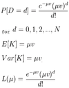
Likelihood function for μ, based on observation of (d, v) is

L(μ; d, v) = e^-μvμ^d

Maximum Likelihood Estimate (MLE) and Maximum Likelihood Estimator for μ given by respectively:

Question 42

Non-Parametric Estimation of Survival Function - Limitations

Answer 42

This empirical approach has limitations:

1. Smoothness of S(t): Estimating S(t) using this empirical approach would result in a step function i.e. S(t) would step down for each t where a death was observed. However, S(t) can be smoothed using statistical techniques.
2. Size of group: It is difficult to find a sufficiently large population to observe easily. A large amount of lives must be observed to provide an accurate estimate of S(t). The larger the population used the less significant the steps become, i.e. each death has less of an impact on S(t), and so the smoother S(t) is expected to become.
3. Time period of observation: This estimation requires the same group of lives to be observed until the last person dies. That means the observation period may be over 100 years. By the end of this period, the data is unlikely to be an appropriate basis on which to model a survival function for the current population. This is because the level of mortality is likely to change in both level and shape over this period e.g. medical advances, improved diet etc. An alternative approach is to use the whole population - using different segments for each age.
4. Censoring: In order to use the approximation for S(t) above, we need to observe each life until it dies. In practice, some of the lives in the observation may disappear from the observation for reasons other than death, for example, emigration. Or, we may not be able to ascertain their exact date of death. This type of issue is referred to as censoring.

Question 43

Forms of Censoring

Answer 43

1. Right-censoring: The observation finishes before the terminal event has necessarily happened for all subjects. For example, the investigation ends on a fixed date.
2. Left-censoring: The observation does not allow us to know when a subject entered into the state we are observing. For example, in bio-medical research it is usually recorded when a patient entered the hospital at a particular date, and that he survived for a certain amount of time thereafter; however, the researcher does not necessarily know, or have on record, when exactly the symptoms of the disease first occurred.
3. Interval-censoring: The observation set-up only allows us to know whether the event fell within some interval of time. It does not allow us to say the exact date of the event. For example, women are tested for cervical cancer every three years. Therefore, if one of the regular tests reveals cancer, it is not possible to pin-point the exact date the cancer developed but it is possible to say that it fell within the three-year period prior to this test.
4. Random censoring: This occurs when a subject ceases to be observed at a random time, before they have experienced the terminal event. For example, a member of a pension scheme transfers their benefits out of the scheme. This transfer would occur at a time which could not have been pre-empted and means the observed lifetime of this member is censored.
5. Informative censoring: Censoring is informative if it gives information about the subject in relation to the terminal event. For example, if an employee of a company retires on the grounds ill-health, one would expect them to have a higher rate of mortality than an employee of the same age who remains at the firm.
6. Non-informative censoring: Censoring is non-informative if it gives no information about the subject or event in question. For example, in survival analysis, if a person in the population emigrates, this does not provide any additional information about the expected lifetime of this person.
7. Type I censoring: This describes the situation when a observation is terminated at a particular point in time, so that the remaining subjects are only known not to have reached the terminal event. For example, in survival analysis we end the observation on a fixed date. In this case, the censoring time is often fixed, and the number of terminal events observed is a random variable.
8. Type II censoring: In contrast to type I censoring, with type II censoring the observation continues until a fixed proportion of the subjects have reached the terminal event. For example, an investigation into the safety of a drug may require a certain level of success to be observed before the drug can be marketed e.g. recovery of 95% of the patients.

Question 44

Kaplan Meier Estimate (Product Limit Estimate)

Answer 44

Suppose we observe a population of size N. Imagine we observe m deaths within this population before terminating our observation. The m deaths occur at k different times. (This allows for some deaths occuring at the same time and clearly k ≤ m.)

Denote the i th observed time of death by t_i, where t₁ < t₂ < …< t_{k - 1} < t_k and 1 ≤ i ≤ k.

Let n_i represent the number of lives at risk and under observation just prior to time t_i, and di, the number of deaths at time t_i.

Let c_i represent the total lives censored between t_i and t_{i + 1}.

The Kaplan-Meier estimate or product limit estimate of the survival function S(t) is:

Question 45

Nelson-Aalen Estimate

Answer 45

Question 46

Cox Model (Proportional Hazards)

Answer 46

The Cox model, also known as the Proportional Hazards model, provides the following format for modelling the hazard function:

Question 47

Define Time Homogeneous Markov Chain

Answer 47

A Markov chain is a stochastic process with discrete states operating in discrete time in which the probabilities of moving from one state to another are dependent only on the present state of the process.

EITHER

If the transition probabilities are also independent of time.

OR

If the l-step transition probabilities are dependent only on the time lag, the chain is said to be time-homogeneous.

Question 48

Categorise Stochastic Models by State Space / Time Space into Continous and Discrete

Answer 48

State Space Discrete + Time Space Discrete

• Markov chain, Markov jump chain, Counting Process, Random Walk
• E.g. No claims bonus

SS Discrete + T Continuous

• Counting Process, Poisson Process, Markov jump process, Compound Poisson Process (with Discrete Jump DBN)
• e.g Number of claims received monitored continuously

SS Continuous + T Discrete

• General random walk, White noise
• e.g. Total amount insured on a certain type of policy valued at end of each month

SS Continuous + T Continuous

• Compound Poisson (with continuous jump dbn), Brownian Motion, Ito Process
• e.g. Value of claims arriving monitored continously

Question 49

Prove The Forward Kolmogorov Differential Equations for a Two State Markov Model from First Principles

Answer 49

Question 50

Forwards/Backwards Kolmogorov Equations for
Two State Markov Model

Answer 50

Question 51

Illness-Death Markov Model Define V_i, W_i, S_i, R_i, D_i, U_i, Likelihood Function and MLE’s

Answer 51

State Space = { Able, Ill, Dead }

• V_i *= Waiting time of life i in the able state
• W_i *= Waiting time of life i in the ill state.
• S_i *= Number of transitions able to ill by life i.
• R_i *= Number of transitions ill to able by life i.
• D_i *= Number of transitions able to dead by life i.
• U_i *= Number of transitions ill to dead by life i.

V = ΣV_i etc.

Transition Intensities:

μ = μ^ad, σ = μ^ai, ρ = μ^ia, ν = μ^id

Likelihood function for these transition intensities is proportional to:

L(μ, ν, σ, ρ) = e^-(μ+σ)νe^-(ν+ρ)wμ^dν^uσ^sρ^r

Question 52

Illness Death Model - MLE Distributions

Answer 52

Question 53

MLE for Poisson Model of Mortality

Answer 53

Question 54

Proof of Poisson MLE Expectation and Variance

Answer 54

Question 55

MLE for Binomial Model of Mortality

Answer 55

Question 56

Proof of Binomial MLE Expectation and Variance

Answer 56

Question 57

Adjusting for Censoring - _tq_x in terms of q_x:

• Constant force of Mortality
• Uniform Distribution of Deaths
• Balducci Assumption

Answer 57

In case of censoring, need to be alble to use an approximation for required _tq_x to make up for effect of censoring, meaning that each life potentially contributes to a different part of the q_x.

Three assumptions can be used to relate _bi-aiq_x+ai to q_x.

• For these calculations, the results are related by (2) < (1) < (3)
• UDD - assumes increasing force of mortality
• Balducci assumption - assumes decreasing force of mortality

Question 58

Initial and Central Exposed to Risk

Answer 58

Initial exposed to risk is required for binomial model, that requires equivalent Bernoulli trials to calculate probability.

Central exposed to risk is equivalent to Markov waiting time, used for Poisson and 2 state Markov.

Question 59

Actuarial Estimate
(of q_x for Binomial)

Answer 59

Definition. The actuarial estimate estimates q_x for the Binomial model, allowing for censoring. It is
defined by:

Question 60

Which Mortality Model to Use: Binomial, Poisson or Two-State?

Answer 60

For normal human mortality all of the models are acceptable, due to the low force of mortality. Hence, life tables, which have traditionally been produced using the Binomial model, have been successfully used for years.

However, the Binomial model tends to be inappropriate in the following circumstances:

• where there is plenty of data: it is usually easier to calculate E^c_x, and therefore use the Poisson or two-state model.
• there is more than one state: the Binomial model does not easily extend to multiple states. Hence the two-state or Poisson models should be used.
• *μ *is not small: The approximation used to calculate E_x for the actuarial estimate is invalid for larger μ. It also results in the loss of valuable information about the time of the transition to another state. The Poisson model is also inappropriate for higher and only the two-state model is appropriate here.

Question 61

Key Ratings Factors Used by Insurance Companies in Policy Pricing

Answer 61

To avoid adverse (anti-)selection by customers, companies must attempt to get all salient information relating to risk (ratings) factors, particularly when competitors use the same information.

Models need to be constructed splitting the general population of insured customers into roughly homogenous groups.

Main Factors:

• age
• sex
• smoker status
• level of underwriting (i.e. medical required in advance)
• duration-in-force
• type of policy (through employer / mortgage etc)
• weight v. height
• units of alcohol per week

Additional Factors:

• sales channel (e.g. demographic for daytime tv v. direct mail etc)
• policy size
• occupation (either directly through having a risky job - e.g. bomb disposal expert, or indirectly by being linked to lifestyle proclivities)
• known impairments / personal health history
• family health history

Question 62

Give the Common Definitions for Age Used in Policies

What are the Three Main Kinds of Rate Interval?

Answer 62

Common definitions of age used in observations:

• Age x last birthday:
  covers [x, x + 1]
• Age x nearest birthday:
  covers [x - 0.5, x + 0.5]
• Age x next birthday:
  covers[x - 1, x]

Three kinds of rate interval:

• life year rate interval
  age label changes on date dependent on life’s birthday only
• calandar year rate interval
  age label changes at a set point in the year - e.g. 1 January
• policy year rate interval
  age label changes on policy anniversary

Age at death will be recorded based on the combination of these two aspects of age and policy rate interval.

Question 63

Principle of Correspondence (for estimates of μ and q)

Answer 63

The principle of correspondence states that:

a life alive at time t should be included inthe exposure for age x at time t if and only if, were that life to die immediately, it would be counted in the death data at age x.

I.E. - a life should only be included in the exposed to risk if it would be included in mortality figures for the same period.

Question 64

Calculating Central Exposed to Risk

Answer 64

In order to calculate the central exposed to risk, precisely we require the following items of data for each life, i, included in the investigation:

• date of birth of life
• date observation of life commenced
• date observation of life ceased
• an indicator to show whether observation of life i ceased due to death

In addition to this information, we require the definition of age to be specified.

For each life we would calculate the following for each relevant age x:

1. the date at which the life entered the observation for age x , i.e. the latest of:
   
   • date at which the life reached age x
   • date observation commenced
2. the date at which the life left the observation for age x i.e. the earliest of:
   
   • date at which the life reached age x+1
   • date observation ceased
3. the difference between 1 and 2

Given this information, we can calculate for each life, by calculating the time spent under observation,
whilst age x. This should be totalled across the investigation, to calculate the total central exposed to risk.

Question 65

Census Approximation of Waiting Times

Answer 65

As the Continuous Mortality Investigation Bureau (CMIB) compiles research based on figures provided by UK / Eire life insurance companies compiled for 1st January, it uses a trapezium rule approximation for approximating the central exposed to risk.

The use of the trapezium rule assumes that population changes gradually over the course of the year - an assumption that may be invalid

Question 66

Estimators of q_x and μ_x - which x do they estimate for?

Answer 66

Question 67

Why Policy Anniversaries May Not Be Uniformly Distributed Throughout the Year

Answer 67

The assumption that policy anniversaries are uniformly distributed throughout the year must be treated with care. This assumption may not hold for several reasons. Such as:

• policy anniversaries may be concentrated around certain points of the year. For example just prior to the end of a tax year.
• policy anniversaries may not be independent of birthdays. For example, customers may take out insurance just prior to a birthday to obtain a lower premium.
• employers who provide life assurance through a group arrangement with the life insurer, will **have **the same policy anniversary for all employees.

Question 68

Breslow’s approximation to the partial likelihood function

Answer 68

Breslow’s approximation to the partial likelihood function

Question 69

Likelihood Ratio Test & Statistic for Nested Cox Models

Answer 69

Can start either with:

• null model - start with no covariates and add one at a time
• full model - start with all covariates and then eliminate ones that are likely to be insignificant

Likelihood Ratio Statistic:

LRS = - 2(L_p - L_p+q), where L_p is maximised log-likelihood for model with p parameters, and L_p+q is for model with p + q parameters

If additional q covariates have no effect, then LRS has asymptotic chi-squared dbn with q degress of freedom.

For q to be considered and improvement, LRS must be over threshold value for confidence level (normally 5%) on q degrees of freedom.

Question 70

Derive _tp_x in terms of μ_x

Answer 70

Question 71

Advantages and Disadvatages of Paramateric Graduation of Mortality Data

Answer 71

Advantages

• The graduated rates will progress smoothly provided the number of parameters is small
• Good for producing standard tables
• Can easily be extended to more complex formualae, provided optimisation can be achieved
• Can fit the same formula to different experiences and compare parameter values to highlight differences between them

Disadvantages

• It can be hard to find a formula to fit well at all ages without having lots of parameters
• Care is required when extrapolating: the fit is bound to be best at ages where we have lots of data and can often be poor at extreme ages.

Question 72

Problems not Picked up by
Chi-Square Goodness of Fit

Answer 72

• long runs of deviation of same signs caused by undergraduation
  
  • solution > grouping of signs test
• a few large deviations balanced by more numerous small deviations
  
  • solution > individual standardised deviation tests
• graduated rates may be too high or low across the whole range, but not by enough to show up in chi-square test
  
  • solution > groups of signs
• results of graduation not smooth
  
  • solution > test using third order differences of graduated rates - if graduation smooth, will be small in comparison to values

Question 73

Define Logarithmic Derivative

Answer 73

For a continuously differentiable function f(x),

Question 74

Scenario Example for Questions on General Issues in Real World Actuarial Modelling

A large company wishes to construct a model of sickness rates among its employees to use in evaluating the present and future financial health of its sick pay scheme.

Outline factors which the company should take into consideration when developing
the model.

Answer 74

• The nature of the existing sickness data the company possesses. The model can only be as complex as the data will allow it to be.
• Whether the company has made any previous attempts to model sickness rates among its employees, and how successful they were.
• The complexity of the model – e.g. whether it should be stochastic or deterministic. More complex models will be costlier to prepare and run, but eventually there may be diminishing returns to additional complexity.
• General trends in sickness at the national level may need to be built in.
• The definition of sickness and level of benefits payable under the scheme.
• Does the company plan to change the characteristics of the employees? For example, does it plan to recruit more mature persons?
• The ease of communication of the model.
• The budget and resources available for the construction of the model.
• Capability of staff. Will outside consultants be required?
• By whom will the model be used? Will they be capable of understanding and using it?
• Does the model need to interface with models of other aspects of the company’s business (e.g. taking data from other systems)?
• The independence of sickness rates should be taken into account e.g. in the event of an
  epidemic claims cannot be considered independent.

Question 75

What is the main advantage of a semi-parametric model over a fully parametric one?

Answer 75

We do not need to know the general shape of the hazard/distribution.

Question 76

What is a Stationary Probability Distribution (w.r.t. Markov Chains)?

Answer 76

Let S be the state space.
We say that {π _j | j∈S} is a stationary probability distribution for a Markov chain with transition matrix P if the following
hold for all j∈S :

Question 77

What are the Main Approaches to Graduating Raw Data?

Answer 77

• using parametric graduation - appropriate when there is lots of data available is available on large populations
• using standard tables - if useful data is scarce and an appropriate standard table exists
• using graphical graduation - where there is little relevant data and no standard table (e.g. for compiling data on newly discovered animals or newly demarcated populations)

Question 78

(Modified) individual standardised deviations test

Answer 78

(Modified) individual standardised deviations test

Under the null hypothesis (same as for the chi-squared test) we would expect individual deviations to be distributed Normal (0,1)

• Only 1 in 20 of the zx should lie above 1.96 or below -1.96 in absolute value
• none should lie above 3 or below 3 in absolute value
• about two thirds of the z_x should lie between −1 and +1

If these are not true, then there is a problem with either individual outliers or the sample as a whole.

Question 79

Gompertz-Makeham
Law of Mortality

Answer 79

The Gompertz–Makeham law states that the death rate is the sum of an age-independent component (the Makeham term, named after William Makeham) and an age-dependent component (the Gompertz function, named after Benjamin Gompertz), which increases exponentially with age.

Where external causes of death are rare (laboratory conditions, low mortality countries, etc.), the age-independent mortality component is often negligible. In this case the formula simplifies to a Gompertz law of mortality.

The Gompertz–Makeham law works well from about 30 to 80 years of age.

At more advanced ages, some studies have found that death rates increase more slowly – a phenomenon known as the late-life mortality deceleration – but other studies disagree.

Question 80

What is a Poisson Process?

Answer 80

A Poisson process with rate λ is a continuous-time integer-valued process Nt, t ≥ 0 with the following properties:

• N₀ = 0;
• N_t has independent increments;
• N_t has stationary increments, each having a Poisson distribution, as follows, for s < t, n = 0, 1, 2, …

Question 81

What is Meant by a Proportional Hazards Model?

Answer 81

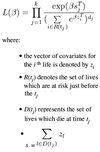
A proportional hazards (PH) model is a model which allows investigators to assess the impact of risk factors, or covariates, on the hazard of experiencing an event.

In a PH model the hazard is assumed to be the product of two terms, one which depends only on duration, and the other which depends only on the values of the covariates.

Under a PH model, the hazards of different lives with covariate vectors z1 and z2 are in the same proportion at all times, for example in the Cox model:

Question 82

What are the Advantages of Using a Cox Model?

Answer 82

Cox’s model ensures that the hazard is always positive. Standard software packages often include Cox’s model.

Cox’s model allows the general ‘shape’ of the hazard function for all individuals to be determined by the data, giving a high degree of flexibility while an exponential term accounts for differences between individuals.

This means that if we are not primarily concerned with the precise form of the hazard, we can ignore the shape of the baseline hazard and estimate the effects of the covariates from the data directly.

The Cox model is included as standard in most statistical modelling software, unlike parametric models, which normally require manual coding and setup.

Question 83

Sum of a Geometric Series of n terms - a + ax + ax² +…ax^n-1

Answer 83

The sum of the first n terms of a geometric series is, where |r|<1

Question 84

General Polynomial Graduation Formula

Describe the general form of the polynomial formula used to graduate the most recent standard tables produced for use by UK life insurance companies.

Answer 84

The general form is

μ_x = αX + exp(βX) ,

where αX takes the form

α₀ + α₁x + α₂x² +…

and βX takes the form

β₀ +β₁x + β₂x² +….

Question 85

Strengths and Weaknesses of the Binomial for Mortality Models

Answer 85

Strengths of Binomial model

• avoids numerical solution of equations
• can be generalised to give the Kaplan-Meier estimate

Weaknesses of Binomial model

• need to compute an initial exposed-to-risk is a pointless complication if census-type data are available
• not so easily generalised as two-state or Poisson models to processes with more than one decrement, and not so easily generalised as two-state model to increments
• estimate of q_x has a higher variance than that of the two-state Poisson models (though the difference is very small unless mortality is very high)

Question 86

Proof that Independent Increments Implies Markov Property

Answer 86

A stochastic process X_(t) operates with state space S. Prove that if the process has independent increments it satisfies the Markov property.