W&M Ch 12 Flashcards
Necessary Criteria for Measures of Credibility
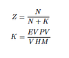
- Z must be greater than or equal to 0 and less than or equal to 1 -No negative credibility and capped at fully credible - 0 ≤ Z ≤ 1 2. Z should increase as the number of risks underlying the actuarial estimate increases (all else equal) 3. Z should increase at a non-increasing rate
Methods for Determining Credibility of an Estimate
-Classical Credibility Approach -Bühlmann Credibility -Bayesian Analysis
Advantage of the classical credibility approach
-Most commonly used and therefore generally accepted -Data required is readily available -Computations are straightforward
Simplifying assumptions about observed experience using Classical Credibility Approach
-Exposures are homogeneous (i.e. same expected number of claims) -Claim occurrence is assumed to follow a Poisson distribution -No variation in the size of loss
Formula for credibility using Bühlmann Credibility
Assumptions using Bühlmann Credibility
-Complement of credibility is given to the prior mean -Risk parameters and risk process do not shift over time -Expected value of the process variance of the sum of N observations increases with N -Variance of the hypothetical means of the sum of N observations increases with N
Desirable Qualities of a complement of Credibility
- Accurate 2. Unbiased 3. Statistically Independent from Base Statistic 4. Available 5. Easy to Compute 6. Logical Relationship to Base Statistic
First Dollar Ratemaking - Products that cover claims for first dollar of loss
- Loss Costs of a Larger Group that Include the Group being Rated 2. Loss Costs of a Larger Related Group 3. Rate Change for the Larger Group Applied to Present Rates 4. Harwayne’s Method 5. Trended Present Rates 6. Competitors’ Rates
Evaluation of Loss Costs of a Larger Group that Include the Group being Rated
-Because data split into classes, believe that experience is different, so combining classes introduces bias and the true expected losses will differ -Not independent because subject experience is included in group experience. However, may not be big issue if subject experience doesn’t dominate the group -Typically is available, easy to compute, and some logical connection
Evaluation of Loss Costs of a Larger Related Group
-Similar to large group including class in that it is biased and true expected mean losses differ –may make adjustment for bias to related experience to match exposure to loss -Is independent- which may make it a better choice than large group including claims -Typically is available, easy to compute, and some logical connection if groups closely related –note: if adjustment made for bias, may be more difficult to compute
Evaluation of Rate Change for the Larger Group Applied to Present Rates
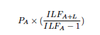
Current Loss Cost of Subject Experience (CLCSE)
- Largely unbiased and likely accurate over the long term assuming rate changes are small
- Independence depends on size of subject experience relative to the larger group
- Typically is available, easy to compute, and logical that rate change of bigger group is indicative of rate change of subject experience

Calculations in Harwayne’s Method
-Compute the state overall means with the base state class distribution -Compute individual state adjustment factors by dividing subject average PP by adjusted related state PP -Multiply each related state’s base class by state adjustment factor to get adjusted state class rates -Complement equals the exposure weighted average of the adjusted related state rates
Evaluation of Harwayne’s Method
-Unbiased as it adjusts for distributional differences -Use of multi-state data generally implies it is reasonably accurate –need enough data to minimize process variance -Mostly independent since subject and related experience from different states -Data is available, but computations can be time consuming -Logical relationship, but may be harder to explain due to calculation complexity
Trended Present Rates
-Current rates should be adjusted for the previously indicated rate, not what was implemented -Changes in loss cost levels –may be due to inflation, distributional shifts, safety advances, etc –trend period (t) taken from original target eff date of current rates to planned eff date
Complement for the Pure Premium Approach

Complement for an indicated rate change when using the Loss Ratio Approach

Evaluation of Trended Present Rates
-Accuracy depends largely on process variance of historical loss costs –primarily used for indications with large amounts of data -Unbiased since pure trended loss costs are unbiased -Independence depends on experience used –if complement comes from a review that used data from 2007-2009 and subject experience is from 2008-2010, then they are not independent -Data is readily available, easy to compute, and is easily explainable
Evaluation of Competitors’ Rates
-Must consider marketing practices and judgment of the competitor and effects of regulation –can cause inaccuracy -Competitors may have different underwriting and claims practices that creates bias -Will be independent -Calculations may be straightforward, but getting data may be difficult -Generally accepted by regulators because of logical relationship –may be the only choice
Excess Ratemaking - Products that cover claims that exceed some attachment point
- Issues -Excess ratemaking deals with volatile lines and low volumes of data -Due to low volume, often use loss costs below attachment point to predict excess losses -Slow development and trend in excess layers can also complicate projections 2. Increased Limits Factors (ILF) 3. Lower Limits Analysis 4. Limits Analysis 5. Fitted Curves
Evlaution of Increased Limits Factors (ILF)
- If subject experience has different size of loss distribution than used in developing ILFs, procedure will be biased and inaccurate, but often best available estimate
- Error associated with estimate tends to be independent of error associated with base statistic
- Data needed incl ILFs and ground-up losses that haven’t been truncated below attachment
- Ease of computation- easiest of the excess complements to compute
- Explainable relationship- controversial; more logically related to losses below attachment point
Evaluation of Lower Limits Analysis
- Even more prone to bias than first method because losses far below attachment point accentuates the impact of variations in loss severity distributions
- Losses capped at lower limit may increase stability and accuracy
- Error associated with estimate tends to be independent of error associated with base statistic
- Data a little more available since losses capped at lower limit
- Ease of computation- just slightly more complex than first method
- Explainable relationship- controversial for same reason as first method

Calculation of Limits Analysis
- Analyze each limit of each coverage separately
- Assume all limits will experience same loss ratio
- Calculate total loss cost (Prem x ELR) for each layer
- Use ILFs to calculate % loss in layer
- Multiply loss cost from layer by calculated %

Evaluation of Limits Analysis
-Biased and inaccurate to same extent as prior two methods, plus assumes LR doesn’t vary by limit -Typically used by reinsurers that don’t have access to the full loss distribution -Calculations are straightforward but take more time than the first two methods -Explainable relationship - controversial for same reason as other methods
Evaluation of Fitted Curves
-Tends to be less biased and more stable, assuming curve replicates general shape of actual data, and significantly more accurate when few claims in excess layer -Less independent due to relience on larger claims to fit curve -Most complex procedure and requires data that may not be readily available -Most logically related to losses in layer, but complexity may make it hard to communicate
