SOA Probability Flashcards
If A ⊂ B then (A n B)
(A n B) = A
Probability Generating Function Defined as PGF where
Px(t) =
Px(t) = E [tX]
E ( X ( X -1 ) ) = 2nd Moment of what Generating Function?
PGF - Probability Generating Function
E [X ∣ j ≤ X ≤ k] - continuous case
Integrate numerator from j to k
( ∫ x ⋅ fX (x) dx )
÷
( Pr ( j ≤ X ≤ k ) )
Percentile for Discrete Random Variables
Fx(πp) ≥ p
i.e the function at πp has to atleast be equal or greater than the percentile p
E [X | j ≤ X ≤ k] - Discrete Case
Sum numerator from x = j to k
( ∑ (x)( Pr [j ≤ X ≤ k] )
÷
( Pr [j ≤ X ≤ k] )
Percentile for Continous Random Variable
density function fX(πp) = p
Has to equal the percentile
Finding mode of discrete random variable
calculate probabilities of each possible value and choose the one that gives the largest probability
Finding mode of continuous random variable
take derivative of density function set it equal to 0 and solve for mode. (finding local maximum of function)
Cumulative Distribution Function (CDF) of a probability density function (PDF)
integrate from lowest value of X to the variable x itself
0 <f></f>
∫ f(t) dt
Chebyshev’s Inequality
Pr( |X-µ| ≥ kσ ) ≤ ( 1 / k2 )
How to break up the inequality of Chebyshev’s Equation
Pr( |X-µ| ≥ kσ )
=
Pr( (X-µ) ≥ kσ ) + Pr( (X-µ) ≤ -kσ )
Univariate Transformation CDF METHOD
From X to Y
1.) Given PDF of X find CDF of X
2.) Perform Transformation where FY( y ) = P( Y ≤ y ) with subsitution
3.) Restate CDF of Y using CDF of X ,
then subsitute CDF of X found in step 1 into CFD of Y
4.) Take Derivative of CDF of Y to find PDF of Y
Univariate Transformation PDF METHOD
From X to Y
1.) Get PDF of X if not given
2.) Find PDF of Y using the formula
fY( y ) = fX( [g-1( y )] ) • | (d/dy) g-1( y ) |
3.) Integrate PDF of Y to get CDF of Y if required
Discrete Uniform PMF
( 1 / b - a + 1)
Discrete Uniform E[X]
( a + b / 2 )
Discrete Uniform Var[X]
[( b - a + 1 )2 - 1]
÷
12
Bernoulli’s E[X]
p
Bernoulli’s Var[X]
pq
Bernoulli’s MGF
pet + q
Bernoull’s Variance Short-cut for Y = (a-b)X + b
(b - a)2• pq
Property of Expected One RV: E[c]=
E[c]=c, c = constant
Property of Expected One RV: E[c⋅g(X)]=
E[c⋅g(X)]= c ⋅ E[g(X)]
Property of Expected One RV: E[g1(X)+g2(X)+…+gk(X)] =
E[g1(X)+g2(X)+…+gk(X)]
=
E[g1(X)] + E[g2(X)]+ …+E[gk(X)]
Variance formula for One RV:
Var[X]
Var[g(X)]
Var[X] = E[(X−μ)2] = E[X2] − (E[X])2
Var[g(X)] = E[(g(X) − E[g(X)])2] = E[g(X)2] − (E[g(X)])2
Property of Variance One RV: Var[c] =
Var[c] = 0,
c = constant
Property of Variance One RV: Var [aX + b]
Var [aX + b] =
a2 • Var[X]
a,b = constant
Coefficient of Variation for One RV
CV[X]=
CV[X] =
(SD[X])
- *÷**
- *(E[X])**
Binomial Mean E[X]
E[X] = np
Binomial Variance Var[X]
Var[X] = npq
Binomial MGF
MX(t) = (pet+q)n
Binomial PGF
PX(t) = (pt+q)n
Hypergeometric PMF: Pr(X = x)
Pr(X = x)
[( m Choose x ) • ( N - m Choose n - x )]
÷
( N choose n )
x = sucess out of m = total sucess
n - x = failures out of N - m = total failures
N = population size; n = sample size
Geometric PMF
Pr(X = x) = (1−p)x−1 • p
Where the first success is observed
Define X as the number of rolls to get
Geometic E[X]
E[X] = ( 1 / p )
Geometric Var[X]
Var[X] = [(1 - p)÷p2]
Geometric MGF
MX(t) =
(pet)
÷
(1−(1−p)et )
for t < −ln(1−p)
Memoryless Property of a Distribution
The memoryless property states that, for positive integer c,
Pr( X − c = x∣ X > c ) =
Pr(X = x )
Negative Binomial PMF
Pr(X = x) =
(x-1 choose r−1) •pr•(1−p)x−r
r = the desired number of “successes”
p = probability of a success
X = number of “trials” until the rth “success”
X represent the number of coin tosses necessary for three heads to occur
Negative Binomial E[X]
E[X] = r ÷ p
Negative Binomial Var[X]
Var[X] = r•( 1−p ÷ p2)
Negative Binomial MGF
MX(t) =
(pet ÷ 1 − (1 − p)et)r
Geometric Distribution for Pr( X ≥ x )
∑ (1-p)x-1 • p
=
(1-p)x-1
Geometric Distribution Derivation
Independent Bernoulli trials
P(X=x)
= Pr( first “success” on xth “trial”)
= Pr (“failure” on the first x-1 “trials” and “success” on xth “trial”)
= Pr( “failure” on the first x-1 “trials”) • Pr( “success” on the xth “trial”)
= (1 - p)x-1 • p
Geometric Alternative Form (failures)
Let Y be the number of “failures” before the first “success”, rather than the number of “trials”
number of “trials” = number of “failures’’ + number of “successes”
X = Y+ 1 ⇒ Y = X − 1
Let Y be the number of rolls before getting...
Negative Binomial Distribution Derivation
Independent Bernoulli Trials
Pr (X = x )
= Pr (rth “success’’ on xth “trial”)
= Pr( r−1 “successes’’ on the first x−1 “trials” ∩ “success’’ on xth “trial” )
= Pr(r−1 “successes’’ on the first x−1 “trials” )•Pr(“success’’ on xth “trial”)
Negative Binomial Alternative Form “failures”
Let Y be the number of “failures” before the rth “success”
= Pr(X − r = y)
= Pr(X = y + r)
Let Y represent the number of tails before getting the third head
Exponential MGF
Mx(t) = ( 1 / 1−θt )
t < (1 / θ)
Exponential Var[X]
X∼Exponential(θ) = θ2
X∼Exponential(λ) = (1 / λ2)
X∼Exponential(θ) E[X]
E[X]; X∼Exponential(θ) = θ
E[X]; X∼Exponential(λ) = λ
Gamma PDF
fX(x) =
(1 / Γ(α)) ⋅ (xα−1/θα) ⋅ e(−x / θ)
if α is a positive integer then
Γ(α) = (α - 1)!
Gamma E[X]
E[X] = αθ
Gamma Var[X]
Var[X] = αθ2
Gamma MGF
MX(t) = (1 / 1−θt)α
Normal Distribution PDF
fX(x)=
[(1 / (σ • sqrt(2π))] •
( e−[((x−μ)^2) / (2 • σ^2)] )
Standard Normal Distribution
fZ(z) =
(1 / sqrt(2π) •
(e−((z)^2) / 2 ) )
Z = ( X - μ ) / ( σ )
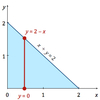
Joint Density Function for Pr( X + Y < 2 )
inner integral limit
double integration:
Determine limits for inner integral following the picture
∫ ( ∫ fX,Y(x,y) dy ) dx
Pr(X ≤ c ∣ Y = y)
Integrate from −∞ to c
∫ fX∣Y(x∣y) dx
=
∫ [fX,Y(x,y) / fY(y)] dx
Pr(X ≤ x ∣ Y ≤ y)
[ Pr(X ≤ x ∩ Y ≤ y)
/ Pr(Y ≤ y) ]
Weighted Average of CDF
FY(y) = a1FC1(y) + a2FC2(y)
Weighted Average of Survival Function
SY(y) = a1SC1(y) + a2SC2(y)
To construct the mixed (or unconditional) distribution of Y
Pr(Y = y)
=
Pr(Y = y∣X = x)⋅Pr(X = x) + Pr(Y = y∣X = x)⋅Pr(X = x)
Pr(A ∣ B) + Pr(A′ ∣ B) =
[ Pr(A∩B) + Pr(A′∩B)
/
Pr(B) ]
Pr(A ∣ B) + Pr(A′ ∣ B) =
[Pr(B)
/
Pr(B) ]
=
1
Double Expectation
E[X] = E[E [X ∣ Y] ]
Law of total Variance
Var[X]
=
E[Var[X | Y]] + Var[E[X ∣ Y]]
EVVE
Pr(X = x∣Y ≤ y) =
Pr(X=x ∩ Y≤y)
/
Pr(Y ≤ y)
Pr(X = x∣Y = y)
Pr(X=x ∩Y=y)
/
Pr(Y=y)
Cov[X,X]
E[X⋅X] − E[X]⋅E[X]
=
E[X2] − (E[X])2
=
Var[X]
Cov[a,X]
0
Cov[a,b]
0
Cov[aX , bY]
ab⋅Cov[X , Y]
Var[aX]
Cov[aX,aX]
=
a2⋅Cov[X,X]
=
a2⋅Var[X]
Cov[X+a , Y+b]
Cov[X , Y]
Cov[aX + bY , cP + dQ]
ac⋅Cov[X,P] + ad⋅Cov[X,Q] + bc⋅Cov[Y,P] + bd⋅Cov[Y,Q]
Var[aX + bY]
a2⋅Var[X] + 2ab⋅Cov[X,Y] + b2⋅Var[Y]
Cov[X,Y] =
E[XY] − E[X]⋅E[Y]
ρX,Y=Corr[X,Y]
Coefficient of Correlation
Cov[X,Y]
/
SD[X]⋅SD[Y]
Multivariate Transformation CDF Method
Case 1: Transforming two variables (X and Y) to one variable (W).
1.) Using equation of transformation, W=g(X,Y), express FW(w)=Pr(W≤w) = Pr[g(X,Y)≤w]
.
- ) Calculate FW(w)=Pr(W≤w) by integrating over region of integration defined by domain of fX,Y(x,y) and g(X,Y)≤w
(transformation) . - ) Differentiate FW(w)
to get fW(w) if required.
Multivariate Transformation PDF Method
Case 2: Transforming two variables (X1 and X2) to two variables (W1 and W2)
1.) Find fX1,X2(x1,x2)
if not given.
- ) Introduce dummy variable (for Case 1 only).
- ) Find inverse of equations of transformation, h1(w1,w2)
and h2(w1,w2)
4.)Calculate determinant of Jacobian matrix, J and take its absolute value
5.) Find fW1,W2(w1,w2) using the following formula.
fW1,W2(w1,w2) = fX1,X2[h1(w1,w2),h2(w1,w2)]⋅|J|, J≠0
Combination Formula
ₙCₖ = [n! / (n-k)! * k!]
Permutation Formula
ₙPₖ = [n! / (n-k)!]
Combinatorial Probability
Probability =(Number of Permutations or Combination Satisfying requirements) / (Total Number of Permutations or Combinations)
