SAS: Base Programming Flashcards

Question 1

Q

Lesson 1: Getting Started with SAS

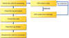
SAS Modes

Answer

A

Interactive

Batch

Noninteractive

Question 2

Q

Lesson 1: Getting Started with SAS

Interactive Mode

Answer

A

Code runs immediately

Question 3

Q

Lesson 1: Getting Started with SAS

Batch Mode

Answer

A

SAS runs the program in the background by submitting it to the operating environment for batch execution.

Program runs when the computer has resources available.

Question 4

Q

Lesson 1: Getting Started with SAS

Noninteractive Mode

Answer

A

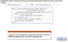
Store store SAS programming statements in a file.

When you issue a SAS command referencing the file, SAS opens, execute the code immediately, and stores any log messages and output in files.

Then SAS closes.

Question 5

Q

Lesson 1: Getting Started with SAS

Types of steps in a SAS program?

Answer

A

Data or Proc

Question 6

Q

Lesson 1: Getting Started with SAS

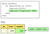
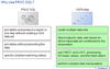
Data Step

Answer

A

A DATA step typically takes data, processes it, and creates a SAS data set, which is data in a form that SAS understands.

A DATA step can create new variables.

Question 7

Q

Lesson 1: Getting Started with SAS

Proc Step

Answer

A

A PROC step typically processes a SAS data set.

PROC steps can generate reports and graphs, manage data, and sort data.

Question 8

Q

Lesson 1: Getting Started with SAS

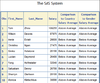
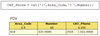
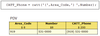
Data read by SAS

Answer

A

Oracle files

SAS data sets

Raw data files

Excel files

Other types of files

Question 9

Q

Lesson 1: Getting Started with SAS

Tasks useful in interactive mode

Answer

A

Debugging programs

Editing programs

Testing programs

Writing programs

Question 10

Q

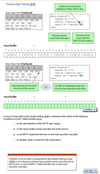
Lesson 2: Navigating and Using the SAS Interface

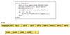
Three main programming windows

Answer

A

Editor window

Log window

Output window

Question 11

Q

Lesson 2: Navigating and Using the SAS Interface

True statements about SAS output

Answer

A

Can create both listing and HTML output

Manage all SAS output in results window

Listing and HTML output are seperate in the results window

Question 12

Q

Lesson 2: Navigating and Using the SAS Interface

Editor Window

Answer

A

Also known as Enhanced Editor

Question 13

Q

Lesson 2: Navigating and Using the SAS Interface

Program Editor Window

Answer

A

Default code editor in operating environments other than Windows

Question 14

Q

Lesson 2: Navigating and Using the SAS Interface

Log Window

Answer

A

Provides messages about your program

Question 15

Q

Lesson 2: Navigating and Using the SAS Interface

Output window

Answer

A

SAS continually adds output to this window

Question 16

Q

Lesson 2: Navigating and Using the SAS Interface

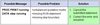
Results vs Output Windows

Answer

A

Results window displays a tree view of output that is created during a SAS session.

Output window is available in all SAS environment.

Question 17

Q

Lesson 2: Navigating and Using the SAS Interface

Are session result preferences stored in SAS program.

Question 18

Q

Lesson 2: Navigating and Using the SAS Interface

What can be done in Explorer window?

Answer

A

Move, copy and delete SAS files

View contents of SAS libraries

Open and create new SAS files

Question 19

Q

Lesson 3: Working with SAS Code

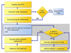
Diagnosing and correcting unbalanced quotation marks

Question 20

Q

Lesson 3: Working with SAS Code

Diagnosing and correcting syntax errors

Question 21

Q

Lesson 3: Working with SAS Code

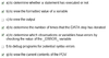
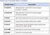
Syntax Error

Answer

A

When programming statements don’t conform to the rules of the SAS language at compile time

Question 22

Q

Lesson 3: Working with SAS Code

Semantic Error

Answer

A

When the language element is correct, but the element might not be valid for a particular usage at compile time

Question 23

Q

Lesson 3: Working with SAS Code

Execution Time Error

Answer

A

When SAS attempts to execute a program and execution fails at execution time

Question 24

Q

Lesson 3: Working with SAS Code

Data Error

Answer

A

When data values are invalid at execution time

Question 25

Q

Lesson 3: Working with SAS Code

Macrorelated Error

Answer

A

When you use the macro facility incorrectly

Question 26

Q

Lesson 3: Working with SAS Code

How SAS compiles and executes

Answer

A

SAS compiles and executes each DATA or PROC step independently based on step boundaries, such as a RUN statement, a QUIT statement, or the beginning of a new DATA or PROC step.

Question 27

Q

Lesson 3: Working with SAS Code

Block Comment

Answer

A

Can appear anywhere a single blank can appear

Cancontain semicolons or unmatched quotation marks

Denoted with /* COMMENT */

Question 28

Q

Lesson 3: Working with SAS Code

Step Boundaries

Answer

A

Run

Quit

Data Statement

Proc Statement

Question 29

Q

Lesson 3: Working with SAS Code

Long running message at top of window indicating that a step is running

Answer

A

Missing run statement or unbalanced quotation marks

Question 30

Q

Lesson 3: Working with SAS Code

A log message indicating that an option seems to be invalid

Answer

A

Missing Semicolon

Question 31

Q

Lesson 3: Working with SAS Code

Log Message indicating that a word wasn’t recognized

Answer

A

Spelling Error

Question 32

Q

Lesson 4: Working with SAS Libraries and SAS Data Sets

SAS Library

Answer

A

Collection of one or more SAS files that are recognized by SAS and that are referenced and stored as a unit

Question 33

Q

Lesson 4: Working with SAS Libraries and SAS Data Sets

Libref

Answer

A

Logical name to reference a SAS library

Question 34

Q

Lesson 4: Working with SAS Libraries and SAS Data Sets

Libraries created at SAS session start

Answer

A

Work: Temporary library

Sasuser: Permanent library

Question 35

Q

Lesson 4: Working with SAS Libraries and SAS Data Sets

Naming a SAS data set

Answer

A

libref. data-set-name
work. data

library_name.data-set-name

Question 36

Q

Lesson 4: Working with SAS Libraries and SAS Data Sets

Libname

Question 37

Q

Lesson 4: Working with SAS Libraries and SAS Data Sets

Assigning Libref

Answer

A

In an interactive SAS session, a libref that you assign with a LIBNAME statement remains assigned until you cancel or change the libref or until you end your SAS session. After you end your SAS session, the contents of a permanent library still exist in their physical location. However, each time you start a new SAS session, you must resubmit a LIBNAME statement to reassign the libref to that permanent library.

Question 38

Q

Lesson 4: Working with SAS Libraries and SAS Data Sets

Proc Contents

Answer

A

View the contents of a SAS library

PROC CONTENTS DATA=libref._ALL_ NODS;

**RUN; **

Question 39

Q

Lesson 4: Working with SAS Libraries and SAS Data Sets

_ALL_ in the PROC CONTENTS

Answer

A

Displays a list of all the SAS files that are in the specified SAS library.

Question 40

Q

Lesson 4: Working with SAS Libraries and SAS Data Sets

NODS in PROC CONTENTS

Answer

A

Default PROC CONTENTS report includes the descriptor portion of each data set in the SAS library.

NODS option to suppress the descriptor portions in the report.

Question 41

Q

Lesson 4: Working with SAS Libraries and SAS Data Sets

Variable

Answer

A

Column in SAS data set

Question 42

Q

Lesson 4: Working with SAS Libraries and SAS Data Sets

Observation

Answer

A

Row in SAS data set

Question 43

Q

Lesson 4: Working with SAS Libraries and SAS Data Sets

Value vs Descriptor

Answer

A

The data portion of a SAS data set contains the data values.

The descriptor portion of a SAS data set contains information about the attributes of the data set and information about each variable.

The information in the descriptor portion is called metadata.

Question 44

Q

Lesson 4: Working with SAS Libraries and SAS Data Sets

Viewing the Descriptor Portion of SAS Data Sets

Answer

A

You can use a PROC CONTENTS step to view the descriptor portion of a data set.

When you specify a single data set in the PROC CONTENTS step and do not include the NODS option, the step creates a report of the descriptor portion for the specified data set.

PROC CONTENTS DATA=SAS-data-set;

RUN;

Question 45

Q

Lesson 4: Working with SAS Libraries and SAS Data Sets

Character Variable

Answer

A

Default Lenth of 1 to 32,767 bytes

Missing values are represented by blanks

Question 46

Q

Lesson 4: Working with SAS Libraries and SAS Data Sets

Numeric Variable

Answer

A

Default length of 8 bytes

Missing values represented by ‘.’

Question 47

Q

Lesson 4: Working with SAS Libraries and SAS Data Sets

Var Statement

Answer

A

Control which variables SAS includes in the Proc Print report

The VAR statement also controls the order in which SAS displays the variables in the report.

PROC PRINT DATA=SAS-data-set;

VAR variable(s);

RUN;

Question 48

Q

Lesson 4: Working with SAS Libraries and SAS Data Sets

NOOBS

Answer

A

BY default, SAS includes the observation numbers in the report.

Suppress the Obs column by using the NOOBS option in the PROC PRINT statement.

PROC PRINT DATA=SAS-data-set NOOBS;

VAR variable(s);

RUN;

Question 49

Q

Lesson 4: Working with SAS Libraries and SAS Data Sets

Viewing the Data Portion of SAS Data Sets

Answer

A

You can use the PRINT procedure to display the data portion of a SAS data set.

Missing values are represented by blanks for character variables and by periods for numeric variables.

PROC PRINT DATA=SAS-data-set;

RUN;

Question 50

Q

Lesson 4: Working with SAS Libraries and SAS Data Sets

PROC SORT

Answer

A

Sorting Observations in SAS Data Sets

By default, replaces the original data set with the sorted data set. OUT= option to create a new output data set instead of replacing the input data set

By default sorts observations in ascending order of the values for the variable or variables listed in the BY statement.

You can use the DESCENDING option to sort on the variable or variables in descending order instead.

SAS treats missing values as the smallest possible values.

PROC SORT DATA=input-SAS-data-set;

 BY BY-variable(s);

RUN;

Question 51

Q

Lesson 4: Working with SAS Libraries and SAS Data Sets

Defining SAS Libraries for Relational Databases

Answer

A

After a database is associated with a libref, you can use a SAS two-level name to specify any table in the database and then work with that table as you would work with a SAS data set.

You use the CLEAR option in the LIBNAME statement to disassociate a libref that was previously assigned. Disassociating a libref disconnects the database engine from the database and closes any resources that are associated with that libref’s connection.

LIBNAME libref engine-name ;

LIBNAME libref CLEAR;

Question 52

Q

Lesson 4: Working with SAS Libraries and SAS Data Sets

Sample Code

Assigning a Libref and Viewing the Contents of the Library

Answer

A

libname orion ‘my-file-path’;

proc contents data=orion._all_nods;
run;

Question 53

Q

Lesson 4: Working with SAS Libraries and SAS Data Sets

Sample Code

Creating Work.NewSalesemps

Answer

A

data work.newsalesemps;
length First_Name $ 12 Last_Name $ 18 Job_Title $ 25;
infile ‘my-file-path\newemployees.csv’ dlm=’,’;
input First_Name $ Last_Name $ Job_Title $ Salary;
run;

Question 54

Q

Lesson 4: Working with SAS Libraries and SAS Data Sets

Sample Code

Displaying the Descriptor Portion of a Data Set

Answer

A

proc contents data=work.newsalesemps;
run;

Question 55

Q

Lesson 4: Working with SAS Libraries and SAS Data Sets

Sample Code

Displaying the Data Portion of a Data Set

Answer

A

proc print data=work.newsalesemps noobs;
var Last_Name First_Name Salary;
run;

Question 56

Q

Lesson 4: Working with SAS Libraries and SAS Data Sets

Sample Code

Sorting a Data Set by Two Variables and Displaying the Output Data Set

Answer

A

proc sort data=work.newsalesemps
out=work.newsalesemps3;
by Job_Title descending Salary;
run;

proc print data=work.newsalesemps3;
run;

Question 57

Q

Lesson 4: Working with SAS Libraries and SAS Data Sets

Steps/statements that create printed output

Answer

A

Proc Print

Proc Contents

Question 58

Q

Lesson 4: Working with SAS Libraries and SAS Data Sets

Temporary Data Set

Answer

A

work.data or data

when specify a one level data set name SAS assumes the library is work and the data set is temp

Question 59

Q

Lesson 5: Creating SAS Data Sets

$w.

Answer

A

writes standard character data.

Question 60

Q

Lesson 5: Creating SAS Data Sets

w.d

Answer

A

writes standard numeric data

Question 61

Q

Lesson 5: Creating SAS Data Sets

COMMAw.d

Answer

A

writes numeric values with a comma that separates every three digits and a period
that separates every decimal fraction.

COMMA7.0 = 12,354

Question 62

Q

Lesson 5: Creating SAS Data Sets

COMMAXw.d

Answer

A

writes numeric values with a period that separates every three digits and a comma
that separates the decimal fraction.

COMMAX7.0 = 12.354

Question 63

Q

Lesson 5: Creating SAS Data Sets

DOLLARw.d

Answer

A

writes numeric values with a leading dollar sign, a comma that separates every three
digits, and a period that separates the decimal fraction.

DOLLAR7.0 = $12,345

Question 64

Q

Lesson 5: Creating SAS Data Sets

EUROXw.d

Answer

A

writes numeric values with a leading euro symbol (€), a period that separates every
three digits, and a comma that separates the decimal fraction.

Answer 61

A

01/01/1960

Answer 62

A

31/12/1960

Answer 63

A

31DEC1959

Answer 64

A

January 1, 1960

Answer 65

A

Friday, January 1, 1960

Answer 66

A

A basic DATA step that contains only a SET statement creates an exact copy of the input SAS data set.

A DATA step can reference temporary or permanent libraries.

Remember that you use a LIBNAME statement to assign a libref to a SAS library.

DATA output-SAS-data-set-name;
SET input-SAS-data-set-name;
RUN;

Answer 67

A

Compilation Phase: SAS scans the step for syntax errors. Then, SAS creates the program data vector (PDV) and the descriptor portion of the output data set. The PDV contains two temporary variables: _N_, which tracks the iterations of the DATA step, and _ERROR_, which signals the occurrence of an error that is caused by the data during execution.
Execution Phase: SAS reads and processes the input data set, and creates the data portion of the output data set.

Answer 68

A

Ccontrols which observations SAS writes to the output data set

WHERE where-expression;

Answer 69

A

DROP: Names the variables to exclude from the output data set

KEEP: Names the variables to include in the output data set

DROP variable-list;

KEEP variable-list;

Answer 70

A

You can assign permanent labels and format to the variables in your output data set to control the way that variables names and values appear in reports.

Labels and formats don’t affect the stored names or values; they are stored in the descriptor portion of the data set.

You use a LABEL statement to assign a label to a variable.

To specify that SAS should display variable labels rather than names in a PROC PRINT report, you use the LABEL
option in the PROC PRINT statement.

You use a FORMAT statement to assign a format to a variable.

Answer 71

A

data work.subset1;
set orion.sales;
where Country=’AU’ and Job_Title contains ‘Rep’;
run;

Answer 72

A

data work.subset1;
set orion.sales;
where Country=’AU’ and Job_Title contains ‘Rep’;
keep First_Name Last_Name Salary Job_Title Hire_Date;
run;

proc print data=work.subset1 label;
run;

Answer 73

A

data work.subset1;
set orion.sales;
where Country=’AU’ and Job_Title contains ‘Rep’;
keep First_Name Last_Name Salary Job_Title Hire_Date;
label Job_Title=’Sales Title’ Hire_Date=’Date Hired’;
run;

Answer 74

A

data work.subset1;
set orion.sales;
where Country=’AU’ and Job_Title contains ‘Rep’;
keep First_Name Last_Name Salary Job_Title Hire_Date;
label Job_Title=’Sales Title’ Hire_Date=’Date Hired’;
format Salary comma8. Hire_Date ddmmyy10.;
run;

Answer 75

A

data work.subset1;
set orion.sales;
where Country=’AU’ and Job_Title contains ‘Rep’;
keep First_Name Last_Name Salary Job_Title Hire_Date;
label Job_Title=’Sales Title’ Hire_Date=’Date Hired’;
format Salary comma8. Hire_Date ddmmyy10.;
run;

proc print data=work.subset1 label;
run;

Answer 76

A

No more observations to read in the input data set.

Answer 77

A

January 1, 1960

Answer 78

A

_N_, which tracks the iterations of the DATA step

_ERROR_, which signals the occurrence of an error that is caused by the data during execution

If there is an Error = 1

Answer 79

A

varianble name or constant

numeric or character

Answer 80

A

arithmetic, logical or comparison

Answer 81

A

descriptor portion of output data set

Program Data Vector: (PDV)

The _N_ and _ERROR_ automatic variables

Answer 82

A

You can use the SAS/ACCESS LIBNAME statement to assign a libref to a Microsoft Excel workbook.

Then, SAS treats each worksheet in the workbook as though it is a SAS data set.

You can use the Explorer window or the CONTENTS procedure to view the worksheets, or you can reference a worksheet directly in a DATA or PROC step.

In SAS, Excel worksheet names contain a dollar sign.

To reference an Excel worksheet directly in a DATA or PROC step, you use a SAS name literal because a valid SAS name cannot contain a dollar sign.

LIBNAME libref ‘physical-file-name’;

Answer 83

A

You can use an Excel worksheet as input data in a DATA step to create a new SAS data set.

You use a SET statement with a SAS name literal to read from an Excel worksheet.

You can also use other DATA step statements such as WHERE, KEEP, DROP, LABEL, and FORMAT statements with input from an Excel worksheet.

Answer 84

A

You can use a PROC IMPORT step to read an Excel worksheet and create a SAS data set from it.

The Import Wizard is a point-and-click interface that generates PROC IMPORT code for you.

PROC IMPORT OUT= output-data-set

** DATAFILE=’input=excel-workbook’**

** DBMS=EXCEL REPLACE;**

** RANGE=’range-name’;**

RUN;

Answer 85

A

You can use the DATA step to create an Excel worksheet from a SAS data set if you use the SAS/ACCESS LIBNAME statement to assign a libref to the Excel workbook that contains the worksheet.

You use one DATA step for each worksheet that you want to create.

LIBNAME libref ‘physical-file-name’;

DATA output-excel-worksheet;

** SET input-data-set;**

RUN;

Answer 86

A

You can use the SAS/ACCESS LIBNAME statement along with the COPY procedure to create an Excel workbook that contains one or more worksheets from one or more SAS data sets.

The COPY procedure creates a worksheet for each SAS data set that is listed in the SELECT statement.

LIBNAME output-libref ‘physical-file-name’;

PROC COPY IN=input-libref OUT=output-libref;

** SELECT input-data-set1 input-data-set2;**

RUN;

Answer 87

A

The Export Wizard is a point-and-click interface that generates PROC EXPORT code for you.

PROC EXPORT DATA= input-data-set

** OUTFILE=’output-excel-workbook’**

** DBMS=EXCEL REPLACE;**

RUN;

Answer 88

A

proc import out=work.subset2a;
datafile=’my-file-path\sales.xls’;
range=”Australia$”n;
getnames=yes;
mixed=no;
scantext=yes;
usedate=yes;
scantime=yes;
run;

Answer 89

A

libname orionxls ‘my-file-path\qtr20007a.xls’;

data orionxls.qtr1_2007;
set orion.qtr2_2007;
run;

data orionxls.qwtr2_2007;
set orion.qtr2_2007;
run;

Answer 90

A

libname orionxls ‘my-file-path\qtr20007b.xls’;

proc copy in=orion out=orionxls;
select qtr1_2007 qtr2_2007;
run;

Answer 91

A

numeric SAS date value with the DATE9. format

Answer 92

A

A raw data file is an external file whose records contain data values that are organized in fields.

Raw data files are not software-specific.

Answer 93

A

File in which the
data values are separated by spaces or other special characters.

Answer 94

A

You can use a DATA step to read input from a raw data file and create a SAS data set from it.

Instead of a SET statement, you use an INFILE statement and an INPUT statement.

The INFILE statement specifies the name and location of the raw data file, and the INPUT statement provides specifications for SAS to read the data values as variables.

You use the DLM= option in the INFILE statement to specify a delimiter if the raw data file uses a character other than a blank space to delimit data values.

Delimited data is also known as list input. Other types of raw data files might contain column input or formatted input.

Raw data files can contain either standard or nonstandard data values.

A raw data file does not contain names for the data fields.

You specify variable names for the values in the INPUT statement, and the names that you use must follow the rules for SAS names.

DATA output-SAS-data-set-name;
INFILE ‘raw-data-file-name’ ;
INPUT specifications;
RUN;

Answer 95

A

Default each variable with a length of 8 bytes (SAS truncates character values that are longer than 8 characters)

You can specify multiple variables in one LENGTH statement.

You can either specify different lengths for each variable that you list in the LENGTH statement or you can specify one length for all of the variables listed.

The LENGTH statement must precede the INPUT statement in a DATA step, because SAS determines variable attributes such as length the first time it encounters a variable.

LENGTH variable(s) $ length;

Answer 96

A

Nonstandard data is data that SAS cannot read without extra instructions.

To read nonstandard data, you use the colon format modifier and an informat in the INPUTstatement.

Informats are similar to formats.

An informat is the instruction that SAS uses to read data values into a variable.

An informat also provides a length for a character variable.

INPUT variable <$> variable <:informat>;

Answer 97

A

Can use a DROP statement or a KEEP statement

Can use FORMAT and LABEL statements to add permanent attributes to your output data

CANNOT use a WHERE statement

Answer 98

A

Instream data is data that you specify within your program

You use a DATALINES statement to read instream data

You use a NULL statement to indicate the end of the input data

You use the INPUT statement for list input to specify that the instream data is delimited with blanks.

You could also use a LENGTH statement before a DATALINES statement to specify lengths for variables within the instream data that are shorter or longer than 8 bytes.

DATA output-SAS-data-set;
INPUT specifications;
DATALINES;
instream data
;
RUN;

Answer 99

A

data work.subset3;
infile ‘my-file-path\sales.csv’ dlm=’,’;
length First_Name $ 12 Last_Name $ 18 Gender $ 1
Job_Title $ 25 Country $ 2;
input Employee_ID First_Name $ Last_Name $ Gender $
Salary Job_Title $ Country $ Birth_Date :date9.
Hire_Date :mmddyy10.;
keep First_Name Last_Name Salary Job_Title Hire_Date;
label Job_Title=’Sales Title’ Hire_Date=’Date Hired’;
format Salary dollar12. Hire_Date monyy7.;
run;

Answer 100

A

data work.subset4;
input Employee_ID First_Name $ Last_Name $;
datalines;
120102 Tom Zhou
120103 Wilson Dawes
120121 Irenie Elvish
;
run;

Answer 101

A

Process of identifying invalid values in your data.

For example, you might have character values stored in a numeric variable.

Or you might have invalid date values such as 99NOV1978.

Invalid data values cause data errors when the program runs.

Answer 102

A

PROC PRINT

PROC FREQ

PROC MEANS

PROC UNIVARIATE

Answer 103

A

You can use a PROC PRINT step with a VAR statement and a WHERE statement to create a report of observations with invalid values.

For example, you can create a report that includes observations that have missing values for a particular variable.

You use a SAS date constant to convert a calendar date to a SAS date value.

PROC PRINT DATA=SAS-data-set;

** VAR variable(s);**

** WHERE where-expression;**

RUN;

Answer 104

A

You cannot use PROC PRINT to detect values that are not unique.

Instead, you can use PROC FREQ to view a frequency table of the unique values for a variable.

You can use the TABLES statement in a PROC FREQ step to specify which frequency tables to produce.

You can use the NLEVELS option to display a table that provides the number of distinct values for each variable named in the TABLES statement.

You can use the NOPRINT option in the TABLES statement to suppress the individual frequency tables.

PROC FREQ DATA=SAS-data-set ;

** TABLES variable(s) ;**

RUN;

Answer 105

A

You can use PROC MEANS to create summary reports of descriptive statistics such as SUM, MEAN, and RANGE

Default statistics for all numeric variables: N, MEAN, STD, MIN, and MAX

PROC MEAN step, such as NMISS, which is the number of observations with missing values

Answer 106

A

PROC UNIVARIATE produces summary reports of descriptive statistics.

In addition, PROC UNIVARIATE produces tables of extreme observations and missing values.

The NEXTROBS= option in the PROC UNIVARIATE statement specifies the number of extreme observations that PROC UNIVARIATE lists.

Answer 107

A

You can use an assignment statement to convert values of a variable.

The assignment statement is one of the few SAS statements that don’t begin with a keyword.

An assignment statement evaluates an expression and assigns the resulting value to a new or existing variable.

variable=expression

Answer 108

A

Converts all letters in an argument to uppercase

UPCASE(argument)

Answer 109

A

By default, an assignment statement in a DATA step applies to every observation in the data set.

To apply different assignment statements to different observations, you can use conditional statements.

The IF-THEN statement executes a SAS statement for observations that meet specific conditions.

IF expression THEN statement;

Answer 110

A

You can use PROC SORT to remove duplicate observations from your data by specifying the NODUPRECS option in the PROC SORT statement.

NODUPRECS checks only consecutive observations, so it’s a good idea to sort by all variables when you use NODUPRECS.

You can use the NODUPKEY option in the PROC SORT statement to remove observations with duplicate BY values.

You can use the EQUALS option along with the NODUPRECS and NODUPKEY options in the PROC SORT statement to maintain the relative order of the observations within the input data set and the output data set.

Answer 111

A

proc print data=orion.nonsales;
var Employee_ID Gender Salary Job_Title Country
Birth_Date Hire_Date;
where Employee_ID = . or
Gender not in (‘F’,’M’) or
Salary not between 24000 and 500000 or
Job_Title = ‘ ‘ or
Country not in (‘AU’,’US’) or
Birth_Date > Hire_Date or
Hire_Date < ‘01JAN1974’d;
run;

Answer 112

A

proc freq data=orion.nonsales nlevels;
table _all_ / noprint;
run;

Answer 113

A

proc means data=orion.nonsales n nmiss min max;
var Salary;
run;

Answer 114

A

proc univariate data=orion.nonsales nextrobs=8;
var Salary;
run;

Answer 115

A

data work.clean;
set orion.nonsales;
Country=upcase(Country);
run;

Answer 116

A

data work.clean;
set orion.nonsales;
Country=upcase(Country);
if Employee_ID=120106 then Salary=26960;
else if Employee_ID=120115 then Salary=26500;
else if Employee_ID=120191 then Salary=24015;
else if Employee_ID=120107 then
Hire_Date=’21JAN1995’d;
else if Employee_ID=12011 then
Hire_Date=’01NOV1978’d;
else if Employee_ID=121011 then
Hire_Date=’01JAN1998’d;
run;

Answer 117

A

proc sort data=orion.nonsalesdupes out=sorted nodupkey
equals;
by Employee_ID;
run;

Answer 118

A

Integrity constraints are data validation rules that you can specify to restrict the data values that can be stored for a variable in a SAS data set.

To eliminate the possibility of invalid data in your data set, you can place integrity constraints on the data set.

Integrity constraints help you preserve the validity and consistency of your data.

When the values associated with an integrity constraint variable are added, updated, or deleted, SAS enforces the integrity constraints.

Answer 119

A

General integrity constraints restrict the values of variables within a single file

Answer 120

A

Limits the data values of variables to a specific set, range, or list ofvalues. Check constraints can also be used to ensure that the data values in one variable within an observation are contingent on the data values of another variable in the same observation.

Answer 121

A

Requires that a variable contain a data value. Null (missing) values are not allowed.

Answer 122

A

Requires that the specified variable or variables contain unique data values. A null data value is allowed but is limited to a single instance.

Answer 123

A

Requires that the specified variable or variables contain unique data values and that null data values are not allowed. Only one primary key can exist in a data file.

Answer 124

A

A referential integrity constraint is created when a primary key integrity constraint in one data file is referenced by a foreign key integrity constraint in another data file.

The foreign key constraint links the data values of one or more variables in the foreign key data file, to corresponding variables and values in the primary key data file.

Data values in the foreign key data file must have a matching value in the primary key data file, or they must be null.

When data is updated or deleted in the primary key data file, the modifications are controlled by a referential action that is defined as part of the foreign key constraint. You can define separate referential actions for the update and delete
operations.

Answer 125

A

Prevents the data values of the primary key variables from being updated or deleted if there is a matching value in one of the foreign key data file’s corresponding foreign key variables.

The restrict type of action is the default action if one is not specified.

Answer 126

A

Enables the data values of the primary key variables to be updated or deleted, but matching data values in the foreign key data files are changed to null (missing) values.

Answer 127

A

Enables the data values in the primary key variables to be updated, and additionally updates matching data values in the foreign key data files to the same value.

The cascade type of action is supported only for update operations.

Answer 128

A

Use in a conditional statement to write the current observation to a specific data set that is listed in the DATA statement.

Tells SAS to write the current observation to a SAS data set immediately, not at the end of the DATA step.

OUTPUT ;

Answer 129

A

The SAS data set Orion.Employee_Addresses contains addresses for all Orion Star employees.

Suppose you want to create three separate data sets based on the value of the variable Country.
If the value of Country is US, write the observation to the USA data set.
If the value of Country is AU, write the observation to the Australia data set.
If the value of Country is anything else, write the observation to the Other data set.

data usa australia other;
set orion.employee_addresses;
if Country = ‘AU’ then output australia;
else if Country = ‘US’ then output usa;
else output other;
run;

Answer 130

A

Suppose you’re reading a raw data file and want to create two data sets based on the value of the automatic temporary variable _ERROR_.

If the observation contains errors, write the observation to the data set Errors.

Otherwise, write the observation to the data set Correct.

data errors correct;
infile ‘sales.csv’ dlm=’,’;
input Employee_ID First $ Last $
Gender $ Salary Job_Title $ Country $
Birth_Date :date9.
Hire_Date :mmddyy10.;
if _ERROR_ = 1 then output errors;
else output correct;
run;

Answer 131

A

Prints a ruler and the raw data record in the log

Assigns a missing value to the variable that the invalid data affects

Prints a note about the error in the log

Prints the variable values in the corresponding SAS observation in the log

Answer 132

A

calculate sample statistics

create SAS date values

convert U.S. ZIP codes to state postal codes

round values

generate random numbers

extract a portion of a character value

convert data from one data type to another

Answer 133

A

Use to perform an action conditionally

The IF/THEN statement executes a SAS statement when the condition in the IF clause is true.

IF expression THEN statement;

To assign the value 26960 to the variable Salary when the value of Employee_ID is 120106, add the following IFTHEN statement to your DATA step.

data work.clean;
set orion.nonsales;
if Employee_ID=120106 then Salary=26960;
run;

Answer 134

A

Suppose you want to assign a value to Salary based on the other possible values of Employee_ID. One way to do this is to add IF/THEN statements for the other two conditions, as shown below:

if Employee_ID=120106 then Salary=26960;
if Employee_ID=120115 then Salary=26500;
if Employee_ID=120191 then Salary=24015;

However, when the DATA step executes, SAS evaluates each IF statement in order, even if the first condition is true.

This wastes system resources and slows the processing of your program.

The ELSE statement must immediately follow the IFTHEN statement in your program.

An ELSE statement executes only if the previous IF/THEN/ELSE statement is false.

data work.clean;
set orion.nonsales;
if Employee_ID=120106 then Salary=26960;
else if Employee_ID=120115 then Salary=26500;
else if Employee_ID=120191 then Salary=24015;
run;

Answer 135

A

LENGTH variable(s) $ length;

Variable name, a dollar sign if it is a character variable, and then the length.

You can specify multiple variables in one LENGTH statement.

Remember that SAS determines variable attributes such as length and type the first time it encounters a variable. So, for the LENGTH statement to define the length for the variables in the output data set, it needs to precede any other references to the variable.

data work.subset3;
infile ‘c:\oriondata\sales.csv’;
length First_Name $ 12 Last_Name $ 18 Gender $ 1;
input Employee_ID First_Name $ Last_Name $
Gender $ Salary Job_Title $ Country $;
run;

Answer 136

A

WHERE whereexpression;

Specifies a condition for selecting observations and can be any valid SAS expression.

An expression is a sequence of operands and operators that form a set of instructions.

Must follow several rules:

Can include variables, constants, or both

Variables must exist in the input data set

Character constants must be enclosed in quotation marks

Numeric constants cannot be enclosed in quotation marks

data work.subset1;
set orion.sales;
where Country=’AU’ and Job_Title contains ‘Rep’;
run;

Answer 137

A

variable=expression;

If the expression in an assignment statement contains a missing value, the result of the expression is also a missing value.

Answer 138

A

SUM(argument1,argument2,…)

Returns the sum of the specified arguments.

If an argument contains a missing value, it ignores the missing value and returns the sum of the non-missing values.

Answer 139

A

MONTH(SAS-date)

You can use SAS date functions in assignment statements to specify SAS date values as part of your expressions or to create SAS date values.

The MONTH function extracts a month from a SAS date value.

Answer 140

A

Remember that you can use a DROP statement or KEEP statement in a DATA step to subset variables in the output data set.

When SAS processes a DROP statement, the variables listed in the DROP statement are included in the PDV.

SAS reads values for those variables into the PDV for each observation, but does not write those variables to the output data set.

Answer 141

A

The DO statement, together with the other SAS statements it contains, is known as a DO group.

Each DO group must end with an END statement.

SAS executes the statements withing the first DO group only if the expression in the IF-THEN statement is true.

SAS executes the statements within the second DO group only if the expression in the first IF expression is false and the expression in the ELSE IF expression is true.

Remember that SAS creates the attributes for a variable, including length, based on the first time it encounters that variable.

You use a LENGTH statement to specify the length for a variable explicitly.

IF expression THEN

** DO;**

** executable statements**

** END;**

ELSE IF expression THEN

** DO;**

** executable statements**

END;

Answer 142

A

The WHERE statement selects observations when they are read from the input data set, so you can’t use the WHERE statement to subset observations based on a variable that you create in the same DATA step.

You can use the subsetting IF statement to subset observations based on the value of a variable you create.

You can specify multiple expressions in a subsetting IF statement.

You cannot use special WHERE operators in IF expressions.

You must use the WHERE statement rather than a subsetting IF statement in a PROC step

You can always use a subsetting IF statement in a DATA step.

You can use a WHERE statement in a DATA step if the expression in the WHERE statement references only variables from the input data set, or from all input data sets if the step uses multiple input data sets.

IF expression;

Answer 143

A

You can use a DELETE statement within an IF-THEN statement as an alternative to the subsetting IF statement.

The DELETE statement is especially useful if it is easier to specify a condition for excluding observations than for selecting observations.

IF expression THEN DELETE;

Answer 144

A

data work.comp;
set orion.sales;
Bonus=500;
Compensation=sum(Salary,Bonus);
BonusMonth=month(Hire_Date);
run;

Answer 145

A

data work.comp;
set orion.sales;
drop Gender Salary Job_Title Country
Birth_Date Hire_Date;
Bonus=500;
Compensation=sum(Salary,Bonus);
BonusMonth=month(Hire_Date);
run;

Answer 146

A

data work.bonus;
set orion.sales;
length Freq $ 12;
if Country=’US’ then
do;
Bonus=500;
Freq=’Once a Year’;
end;
else if Country=’AU’ then
do;
Bonus=500;
Freq=’Twice a Year’;
end;
run;

Answer 147

A

data work.december;
set orion.sales;
BonusMonth=month(Hire_Date);
if Country=’AU’ and BonusMonth=12;
Bonus=500;
Compensation=sum(Salary,Bonus);
run;

Answer 148

A

Value Extracted: the year

Value Returned: a fourdigit year

QTR(SASdate)
the quarter a number from 1 to 4
MONTH(SASdate)
the month a number from 1 to 12
DAY(SASdate)
the day of the month a number from 1 to 31
WEEKDAY(SASdate)
the day of the week a number from 1 to 7 (1=Sunday, 2=Monday, and so on)

Answer 149

A

Value Extracted: the quarter

Value Returned: a number from 1 to 4

Answer 150

A

Value Extracted: the month

Value Returned: a number from 1 to 12

Answer 151

A

Value Extracted: the day of the month

Value Returned: a number from 1 to 31

Answer 152

A

Value Extracted: the day of the week

Value Returned: a number from 1 to 7 (1=Sunday, 2=Monday, and so on)

Answer 153

A

SAS Date Value Created: the current date

Answer 154

A

SAS Date Value Created: a date with numeric month, day, and year

Answer 155

A

DATA= data set variables are not in the BASE= data set: Drops the variable not present in the BASE=data set.

DATA= data set variables have a different type than the variables in the BASE= data set: Replaces all values for the variable in the DATA= data set with missing values + keeps the variable type of the variable specified in the BASE= data set.

DATA= data set variables are longer than the variables in the BASE= data set: Truncates values from the DATA= data set to fit them into the length that is specified in the BASE= data set.

Answer 156

A

Places the observations from one or more data sets below or above the observations in another data set.

Three methods of combining data vertically: appending, concatenating, and interleaving.

Appending and concatenating data sets both place observations from one data set after the observations from another data set in a single data set.

In both methods, the observations in the combined data set are in the same order that they were in each original data set.

Answer 157

A

When you append data sets, you can only use two input data sets.

Appending adds all of the observations from the second data set to the end of the first data set.

Answer 158

A

Concatenating copies all of the observations from the first data set and all of the observations from the second data set and writes them to a new data set.

Answer 159

A

Interleaving intersperses the observations from two or more input data sets based on the value of one or more common variables, in a new data set.

Answer 160

A

PROC APPEND adds the observations from one SAS data set to the end of another SAS data set.

BASE= names the data set to which the observations are added, and DATA= names the data set containing observations that are added to the base data set.

Can specify only two data sets.

When SAS processes a PROC APPEND step, SAS does not read the observations in the base data set.

SAS cannot change any variable information in the descriptor portion of the base data set.

The base data set has the same number of variables before and after appending.

When the DATA= data set contains variables that are not in the BASE= data set, you can use the FORCE option to force SAS to append the observations.

The FORCE options causes SAS to drop the extra variables in the DATA= data set, and then to issue a warning message to the log.

PROC APPEND BASE=SAS-data-set
DATA=SAS-data-set ;
RUN;

Answer 161

A

When you specify multiple data sets in the SET statement, SAS combines them into a single data set.

In the combined data set, the observations appear in the order in which the data sets are listed in the SET statement.

You can add additional DATA step statements, such as an assignment statement to create new variables in the output data set.

Because the DATA step creates a new data set, the input data sets can contain different variables.

If the data sets specified in the SET statement have a variable with the same name but different types, SAS generates a compile-time error by default.

**DATA SAS-data-set;
SET SAS-data-set1 SAS-data-set2 …;

RUN;**

Answer 162

A

You can use the RENAME= option to change the name of one or more variables.

If the RENAME= option is associated with an input data set in the SET statement, it renames one or more variables being read from that data set.

However, the RENAME= option does not rename variables in the input data set. Instead, the RENAME= option tells SAS which slot in the PDV to use when SAS is building observations from the new data set.

You can use multiple RENAME= options in one SET statement if you want to rename variables from multiple data sets.

SAS-data-set (RENAME=(old-name-1 = new-name-1
old-name-2 = new-name-2
…
old-name-n = new-name-n))

Answer 163

A

Use a DATA step with a BY statement. The BY statement specifies one or more BY variables. SAS uses the values of the BY variables to arrange the observations in the output data set.

Any BY variable that you specify must be common to all input data sets.

By default, SAS arranges observations in ascending order unless you specify the DESCENDING option.

Before you run a DATA step that contains a BY statement, your input data sets must be sorted on the BY variables.

SAS outputs observations with duplicate BY values in the order in which the data sets are listed in the SET statement.

If duplicate values are in the same data set, SAS outputs those observations in the order in which they appear in the data set.

You could also interleave data sets by concatenating them first, and then sorting the output file.

DATA SAS-data-set;
SET SAS-data-set1 SAS-data-set2 …;
BY BY-variable(s);

RUN;

Answer 164

A

proc append base=emps
data=emps2010 force;
run;

Answer 165

A

data empsall2;
set empscn empsjp(rename=(Region=Country));
run;

Answer 166

A

data empsname;
set empscn empsjp(rename=(Region=Country));
by First;
run;

Answer 167

A

When you combine data sets horizontally, you combine the observations from multiple data sets into a single observation in a new data set.

To combine data sets horizontally, it’s important to understand the relationship between the input data sets.

The relationships between input data sets can be one-to-one, one-to-many, many-to-one, many-to-many, or non-matching.

Answer 168

A

Combines observations from two or more data sets into a single observation in a new data set.

Answer 169

A

Merging that is based on the values of one or more common variables.

Answer 170

A

To match-merge using the DATA step, you use the MERGE and BY statements.

The MERGE statement joins observations from two or more SAS data sets into single observations.

The BY variables must be common to all input data sets, and the input data sets must be sorted on the BY variables.

If you specify only one data set in the MERGE statement, SAS treats the MERGE statement like a SET statement.

When you match-merge data sets that have a one-to-one relationship, the output data set has the same number of observations as the input data sets.

DATA SAS-data-set;

** MERGE SAS-data-set1 SAS-data-set2 … ;**

** BY BY-variable(s);**

RUN;

Answer 171

A

To match-merge data sets that have one-to-many or many-to-one relationships, you use a DATA step with the MERGE and BY statements. T

he DATA step is the same as the one you use to match-merge data sets that have a one-to-one relationship.

A BY group is a group of observations that have the same value of the BY variable.

When the input data sets have a one-to-many or many-to-one relationship, each BY group might contain more than one observation.

The output data set contains all of the observations for each BY group.

Answer 172

A

Use the DATA step with the MERGE and BY statements.

The DATA step is the same as the one you use for match-merging data sets with other relationships.

The output data set contains both matches (observations that contain data from both input data sets) and non-matches (observations that contain data from only one input data set).

When you specify the IN= data set option after an input data set in the MERGE statement, SAS creates a temporary variable that indicates whether the data set contributed data to each output observation.

You can specify the IN= option for multiple input data sets in one MERGE statement.

To create an output data set that contains only matches or only non-matches, you can use the IN= data set option to identify which input data sets contributed data to each observation that SAS outputs.

Then, you can use the subsetting IF statement to output only those observations that contain data from all the input data sets.

SAS-data-set (IN=variable)

Answer 173

A

You can match-merge data sets that have a many-to-many relationship in two ways: using the DATA step techniques that you’ve already learned, or using the SQL procedure.

When you use a DATA step with MERGE and BY statements to match-merge data sets that have a many-to-many relationship, the output data set does not contain all possible combinations.

When you use PROC SQL to join data sets that have a many-to-many relationship, the output data set does contain all possible combinations of matching observations.

Answer 174

A

data empsauc;
merge empsau
phonec;
by EmpID;
run;

Answer 175

A

data empsauc;
merge empsau(in=Emps)
phonec(in=Cell);
by EmpID;
if Emps=0 or Cell=0;
run;

Answer 176

A

SAS system options are instructions that affect your SAS session.

All SAS system options have default settings that SAS uses unless you specify otherwise.

When you create a report, the appearance of the output is determined, in part, by the settings of SAS system options.

You can change the settings of SAS system options to alter the way your reports look.

Many of the SAS system options for procedure output affect only listing output—not HTML output.

Answer 177

A

Global statement to modify SAS system options.

Changed settings of SAS system options remain in effect until you change the settings again or until you end your SAS session.

OPTIONS option(s);

Answer 178

A

Specifies whether or not the date and time appear at the top of your listing output.

Answer 179

A

Specifies whether or not the page number appears at the top of listing output.

Answer 180

A

Specifies the number of lines in a page of listing output.

The PAGESIZE = option has the alias PS=.

Answer 181

A

Specifies the number of characters in a line.

The LINESIZE= option has the alias LS=.

Answer 182

A

Specifies whether the output is centered or left-aligned.

Answer 183

A

Whether or not SAS updates the date and time on every report you create in the same SAS session.

Answer 184

A

Specifies the beginning page number for the next page of output.

Answer 185

A

By default, SAS adds a standard title to reports.

You can use the TITLE/FOOTNOTE statements to specify a title/footnote other than the standard SAS title/no footnote.

They are global statements

You can specify up to 10 titles and 10 footnotes.

Titles and footnotes appear in both listing output and HTML output.

N can be 1 to 10 and indicates the line on which the title or footnote appears. Defaults is line 1.

TITLE ‘text’;
FOOTNOTE ‘text’;

Answer 186

A

Titles and footnotes that you assign remain in effect until you change them, cancel them, or end your SAS session.

To cancel a title or footnote, you issue a TITLE or FOOTNOTE statement with the same number as the existing title or footnote and no text; this also cancels any higher-numbered titles or footnotes.

To cancel all previously defined titles or footnotes, you can specify a null TITLE or FOOTNOTE statement, which has no number and no text.

Answer 187

A

You can change the appearance of variable names in your reports by specifying temporary labels with the LABEL statement in your PROC steps.

When you use a LABEL statement within a PROC step, the label applies only to the PROC step that it’s part of.

Remember that to display labels in PROC PRINT reports, you must use the LABEL option in the PROC PRINT statement

You can assign a temporary label to a variable that already has a permanent label associated with it.

The temporary label always overrides the permanent label in reports.

Answer 188

A

Control how values appear in reports by specifying temporary SAS formats with the FORMAT statement in your PROC steps.

Assign a temporary format to a variable that already has a permanent format associated with it.

In reports, the temporary format always overrides the permanent format.

Answer 189

A

Another way to tell SAS to display labels is to add the SPLIT= option in the PROC PRINT statement.

The SPLIT= option specifies a split-character that indicates where to wrap the label in the report.

SPLIT=’split-character’

Answer 190

A

Use the PROC FORMAT step to create your own formats.

You can define only one format in a VALUE statement, but you can include multiple VALUE statements in one PROC FORMAT step.

The names that you specify for your formats must follow the rules for SAS names.

Do not put a period after the format name in the VALUE statement, but you do put a period after the format name in the FORMAT statement.

You apply your formats in a reporting PROC step, such as a PROC PRINT step, by using a FORMAT statement. You can specify both user-defined formats and SAS formats in the same FORMAT statement.

PROC FORMAT;
VALUE format-name value-or-range1=’formatted-value1’
value-or-range2=’formatted-value2’
…;
RUN;

Answer 191

A

You can use the keyword HIGH to specify the highest possible value of a variable.

You can use the keyword LOW to specify the lowest possible value of a variable.

For character variables, the LOW keyword treats missing values as the lowest possible values. For numeric values, LOW does not include missing values.

Answer 192

A

Selecting only some of the observations

Use the WHERE statement in a PROC step to subset observations in a report.

When you use the WHERE statement, your output contains only the observations that meet the conditions specified in the WHERE expression.

Answer 193

A

Grouping observations by the values of one or more variables.

You can use the BY statement in reporting procedures to group observations in reports.

In a PROC step, the BY statement produces separate sections of the report for each BY group.

Answer 194

A

options dtreset pageno=1;

title ‘Orion Star Sales Salaries’;
footnote3 ‘Confidential’;

proc print data=orion.sales;
var Employee_ID First_Name Last_Name Salary;

run;

title;
footnote;

Answer 195

A

proc print data=orion.sales split=’*’;
var Employee_ID Job_Title Salary;
label Employee_ID=’Sales ID’
Job_Title=’Job Title’
Salary=’Annual*Salary’;
format Salary dollar10.0;
run;

Answer 196

A

proc format;
value $ctryfmt ‘AU’ = ‘Australia’
‘US’ = ‘United States’
other= ‘Miscoded’;
value tiers low-<50000 = ‘Tier 1’
50000-100000 = ‘Tier 2’
100000-high= ‘Tier 3’;
run;

proc print data=orion.sales label;
var Employee_ID Salary Country Hire_Date;
label Employee_ID=’Sales ID’
Hire_Date=’Hire Date’;
format Salary dollar10.0
Hire_Date monyy7.
Country $ctryfmt.
Salary tiers.;
run;

Answer 197

A

proc print data=orion.sales;
var Last_Name Job_Title Country Salary;
format Salary dollar10.0
where Salary>75000;
title ‘Sales Salaries Over $75,000’;
run;

title;

Answer 198

A

proc print data=orion.sales;
by Country descending Gender;
run;

Answer 199

A

Assign descriptive labels to one or more variables.

Element 1: variablen which specifies the name of the variable that you want to label.

Element 1: ‘labeln’ which specifies a label of up to 256 characters, including blanks. Enclose the label in quotation marks.

If the LABEL statement appears in a PROC step, it is temporary and applies only to the PROC step in which it appears.

LABEL variable1=’label1’
;

Answer 200

A

A format is an instruction that SAS uses to display data values.

To make data values more understandable when they are displayed in your procedure output, you can use the FORMAT statement to associate formats with variables.

Formats affect only how the values appear in the output, not the actual data values as they are stored in the SAS data set.

The FORMAT statement has the following elements:

Element 1: variable(s) - specifies one or more variables for SAS to associate with a format.

Element 2: format specifies a SAS format or a userdefined format that is used to write the values of the variables.

You can associate multiple formats with variables in the same FORMAT statement.

If the FORMAT statement appears in a PROC step, it is temporary and applies only to the PROC step in which it appears.

FORMAT variable(s) format;

Answer 201

A

Select observations from SAS data sets that meet a particular condition.

Specifies a condition for selecting observations and can be any valid SAS expression.

An expression is a sequence of operands and operators that form a set of instructions.

A whereexpression must follow several rules:

Rule 1: Can include variables, constants, or both.

Rule 2: Variables in the whereexpression must exist in the input data set.

Rule 3: Character constants must be enclosed in quotation marks.

Rule 4: Numeric constants cannot be enclosed in quotation marks.

WHERE whereexpression;

Answer 202

A

You can use the BY statement to specify variables that are used for grouping.

The BY statement has the following elements:

Element 1: BYvariable(s) specifies one or more variables that the procedure uses to form BY groups. Separate multiple variables by using blanks.

Element 2: the DESCENDING keyword specifies that the observations be sorted in descending order by the specified variable(s)

BY BYvariable(s);

Answer 203

A

The Output Delivery System (ODS) gives you greater flexibility in generating, storing, and reproducing the output from SAS procedures and the DATA step.

Each file format that you can create has a corresponding ODS destination.

To create a certain type of output, you open the destination that is associated with that output type.

When you are finished using a destination, you can close it again.

The default ODS destination is the LISTING destination.

Another ODS destination is the HTML destination.

SAS provides many other ODS destinations such as PDF, RTF, and several destinations that create files that you can open in Excel: CSVALL, MSOFFICE2K, and EXCELXP.

You use the ODS statement to open the destination for each type of formatted output you want to create.

To close a destination, you add the keyword CLOSE to the ODS statement, after the destination.

If you do not close a destination, it remains open until the end of the SAS session.

ODS destination;
ODS destination CLOSE;

Answer 204

A

You can view HTML files in the Results Viewer in SAS, or in Web browsers.

You can view and work with PDF files in Adobe software products. You can view and work with RTF files in word processors.

You use the ODS statement to specify the file that you want to create.

You can open one destination at a time, or you can open multiple destinations at once by using several ODS statements.

You can close all destinations in a single ODS statement by adding the _ALL_ keyword instead of a keyword for a specific destination.

However, if you close all of the destinations, SAS cannot display output for any procedures.

ODS destination FILE=’file-specification’;
ODS _ALL_ CLOSE;

Answer 205

A

A style definition describes how to display the presentation aspects of SAS output such as colors and fonts.

By default, the HTML destination uses the Default style definition, the PDF destination uses the Printer style destination, and the RTF destination uses the RTF style definition.

You cannot apply style definitions to listing output.

To specify a style definition for the output, you can add the STYLE= option to your ODS statement.

ODS destination FILE=’file-specification’
STYLE=style-definition;

Answer 206

A

Creates a CSV file that you can view in the SAS Program Editor window or another text editor as well as in Excel.

Answer 207

A

Creates an HTML file that you can view in a Web browser, Microsoft Word, or Microsoft Excel.

Answer 208

A

Creates an XML file that you can open in Microsoft Excel

Answer 209

A

ods html file=’my-file-path\myreport.html’ style=sasweb;
ods pdf file=’my-file-path\myreport.pdf’;
ods rtf file=’my-file-path\myreport.rtf’;
ods csvall file=’my-file-path\myexcel.csv’;

proc freq data=orion.sales;
tables Country;
run;

ods close _all_;
ods listing;

Answer 210

A

Four statistics for each value, by default: frequency, percent, cumulative freqency, and cumulative percent.

Answer 211

A

Summarize data for two or more categorical variables by showing the number of observations for each combination of
variable values.

Crosstabulation tables are also called contingency tables. The simplest crosstabulation table is a two-way frequency table.

Four statistics appear by default: frequency, percent, row percentage, and column percentage.

Row/observation is listed on the side

Column/Variable is listed on top

Answer 212

A

Produces a series of two-way tables, with a separate table for each level of the other variable

To create an n-way crosstabulation table for two or more variables, you specify an asterisk instead of a space between the variable names in the TABLES statement.

The first variable specifies the table rows and the second variable specifies the table columns.

Answer 213

A

When you use PROC FREQ to create summary reports, it’s more useful to display the distribution of values for some variables than for others.

Frequency distributions work best with variables whose values are categorical and are best summarized by counts instead of averages.

A PROC FREQ report contains a one-way frequency table for each variable that you specify in the TABLES statement.

You can use other statements such as the WHERE statement, the LABEL statement, and the FORMAT statement, within a PROC FREQ step.

Also add options to your PROC FREQ statement, such as the NLEVELS option, the PAGE option, or the COMPRESS option.

Options that you can specify in the TABLES statement include the following: NOPRINT, NOCUM, NOPERCENT, NOFREQ, NOROW, NOCOL, LIST, CROSSLIST, and FORMAT=.

**PROC FREQ DATA=SAS-data-set ;
           TABLES variable(s) ;

RUN;**

Answer 214

A

To create a data set that contains frequencies and percentages, you add the OUT= option to the TABLES statement.

The OUT= option names an output data set that contains the frequency counts and percentages for a frequency table or crosstabulation table.

If the TABLES statement specifies variables for more than one table, the contents of the OUT= data set correspond to the last table specified.

The output data set named in the OUT= option contains two variables that PROC FREQ creates automatically: COUNT and PERCENT.

You can also specify additional options in the TABLES statement to include other frequency and percentage variables in the output, such as the OUTCUM or OUTPCT options.

When you specify the OUT= option in the TABLES statement, PROC FREQ still creates a PROC FREQ report by default, unless you include the NOPRINT option in the PROC FREQ statement.

TABLES variable(s) / OUT=SAS-data-set );

Answer 215

A

Another way to create output data sets is to add an OUTPUT statement that contains the OUT= option to your PROC FREQ step.

There are many options available for specifying statistics in the OUTPUT statement.

If your TABLES statement specifies multiple tables, the contents of the OUTPUT data set correspond to the last table.

If you use multiple TABLES statements, the contents of the OUTPUT data set correspond to the last TABLES statement.

To create multiple output data sets, you can add the OUT= option to both the TABLES statement and the OUTPUT statement in a PROC FREQ step.

OUTPUT OUT=SAS-data-set ;

Answer 216

A

Computes descriptive statistics for continuous numeric variables across all observations and within groups of observations

To calculate statistics for groups of observations use the CLASS statement.

The CLASS statement specifies variables that PROC MEANS uses to group the data.

The variables listed in the CLASS statement are also called classification variables or class variables.

Each combination of class variable values is called a class level.

You can include statistic keywords in the PROC MEANS statement to control the statistics that PROC MEANS displays.

When you specify one or more statistics in the PROC MEANS statement, PROC MEANS does not produce the default statistics.

You can use other options in the PROC MEANS statement, such as NONOBS, MAXDEC=, and FW=.

You can use additional statements such as the WHERE statement, the FORMAT statement, and the TITLE statement.

PROC MEANS DATA=SAS-data-set ;
VAR analysis-variable(s);
CLASS classification-variable(s);

RUN;

Answer 217

A

Use to calculate statistics for groups of observations

Specifies variables that PROC MEANS uses to group the data

The variables listed also called classification variables or class variables.

Each combination of class variable values is called a class level.

Answer 218

A

Provides data summarization tools to compute descriptive statistics for variables across all observations and within groups of observations.

By default PROC SUMMARY does not produce a report

If you omit the VAR statement from a PROC SUMMARY step, PROC SUMMARY produces a simple count of observations.

PROC SUMMARY DATA=SAS-data-set ;
VAR analysis-variable(s);
CLASS classification-variable(s);
RUN;

Answer 219

A

To create an output data set add an OUTPUT statement that contains the OUT= option to the PROC MEANS step.

The output data set that PROC MEANS creates contains several types of variables, including any BY variables, class
 variables, and the automatic variables \_TYPE\_ and \_FREQ\_.

Suppress the display of the PROC MEANS report by using the NOPRINT option in the PROC MEANS step.

Restrict your output data set to only the observations that have the highest _TYPE_ value by using the NWAY option in the PROC MEANS statement.

You can sort the output data set by _TYPE_ values in descending order by using the DESCENDTYPES option in the PROC MEANS statement.

You can use the CHARTYPE option to specify that the values of _TYPE_ be character values.

OUTPUT OUT=SAS-data-set ;

Answer 220

A

PROC TABULATE displays descriptive statistics in tabular format by using some or all of the variables in a data set.

Reports contain one-, two-, or threedimensional tables that contain variables and statistics.

Must specify at least one class variable or one analysis variable. You can also specify both.

A class variable can be character or numeric and it usually has only a few distinct values.

An analysis variable must be numeric and it often contains continuous values.

Four statements are commonly used: #1 PROC TABULATE; #2 CLASS statement, #3 VAR statement, #4 TABLE statement.

The TABLE statement contains from one to three dimension expressions that define a table

The number of dimension expressions that you specify determines the dimensionality of the table in the report.

You can use multiple TABLE statements in one PROC TABULATE step.

Note that the TABLE statement is different from the TABLES statement in a PROC FREQ step.

You can use various operators in a dimension expression.

An asterisk creates categories from the combination of class variable values, which is called crossing.

Blank places the output for the next element immediately after the output for the prior, which is called concatenation.

Displays different statistics in a table by default, depending on whether the table contains any analysis variables.

In a dimension expression, you can specify statistics instead of or in addition to the default statistics.

You use the asterisk operator to attach one or more statistic keywords to a variable or combination of variables.

To summarize all categories, you can specify the special class variable ALL to dimension expressions in a TABLE statement.

**PROC TABULATE DATA=SAS-data-set ;
CLASS classification-variable(s);
VAR analysis-variable(s);
TABLE page-expression,
row-expression,
column-expression ;

RUN;**

Answer 221

A

Create an output data set that contains summary statistics by using the OUT= option in the PROC TABULATE statement.

The OUT= option creates a single data set regardless of the number of TABLE statements in the step.

The output data set that PROC TABULATE creates contains any BY variables; any class variables; the automatic variables _TYPE_, _PAGE_, and _TABLE_; and statistics.

PROC TABULATE DATA=SAS-data-set
OUT=SAS-data-set ;

Answer 222

A

proc format;
value $ctryfmt ‘AU’=;’Australia’
‘US’=’United States’;

ods rtf file=’my-file-path\myprocfreq.rtf’ style=sasweb;

proc freq data=orion.sales;
tables Gender*Country;
where Job_Title contains ‘Rep’;
format Country $ctryfmt.;
title ‘Sales Rep Frequency Report’;
run;

ods rtf close;

Answer 223

A

proc freq data=orion.sales nlevels;
tables Gender Country Hire_Date / noprint;
format Hire_Date date10.;
run;

Answer 224

A

proc freq data=orion.sales noprint;
tables Gender Country / out=freq1;
run;

proc freq data=orion.sales;
tables Gender*Country / out=freq2
outpct;
run;

Answer 225

A

proc freq data=orion.sales;
tables Gender Country / chisq out=freq6 outcum;
output out=freq5 chisq;
run;

Answer 226

A

proc means data=orion.sales sum mean range maxdec=0;
          var Salary;
          class Gender Country;
 run;

Answer 227

A

proc means data=orion.sales noprint;
           var Salary;
           class Gender Country;
           output out=means1;
 run;

proc print data=means1;
run;

Answer 228

A

proc tabulate data=orion.sales;
           class Job\_Title Gender Country;
           var Salary;
           table Country;
           table Job\_Title, Gender, Country;
           table Country\*Salary;
 run;

Answer 229

A

proc tabulate data=orion.sales
                     out=tabulate1;
           class Job\_Title Gender Country;
           var Salary;
           table Country;
           table Job\_Title, Gender, Country;
           table Country\*Salary;
 run;

Answer 230

A

proc freq data=orion.sales;
tables Gender / chisq out=genderfreq outcum;
output out=genderchi chisq;
run;

proc freq data=orion.sales;
tables Country / chisq out=countryfreq outcum;
output out=countrychi chisq;
run;

data allfreq;
length Value $ 7;
set genderfreq(in=gf) countryfreq(in=cf)
genderchi(in=gc) countrychi(in=cc);
if gf then Value=Gender;
else if cf then Value=Country;
else if gc then Value=’Gender’;
else if cc then Value=’Country’;
label _PCHI_=’ChiSquare’
P_PCHI=’PValue’;
keep Value COUNT PERCENT _PCHI_ P_PCHI;
run;

proc print data=allfreq label;
run;

Answer 231

A

proc means data=orion.sales noprint;
 var Salary;
 class Gender Country;
 output out=work.means mean=aveSalary;
 run;

data gender_summary(keep=Gender aveSalary)
country_summary(keep=Country aveSalary);
set work.means;
if _type_=1 then output country_summary;
else if _type_=2 then output gender_summary;
run;

proc sort data=orion.sales out=sort_country;
by Country;
run;

data detail_country;
merge sort_country
country_summary(rename=(aveSalary=CountrySalary));
by Country;
run;

proc sort data=detail_country out=sort_gender;
by Gender;
run;

data detail_country_gender;
merge sort_gender
gender_summary(rename=(aveSalary=GenderSalary));
by Gender;
if Salary>CountrySalary then CS=’Above Average’;
else CS=’Below Average’;
if Salary>GenderSalary then GS=’Above Average’;
else GS=’Below Average’;
label CS=’Comparison*to Country*Salary Average’
GS=’Comparison*to Gender*Salary Average’;
run;

proc sort data=detail_country_gender;
by Employee_ID;
run;

proc print data=detail_country_gender split=’*‘;
var First_Name Last_Name Salary CS GS;
run;

Answer 232

A

twosided confidence limit for the mean

Answer 233

A

corrected sum of squares

Answer 234

A

coefficient of variation

Answer 235

A

onesided confidence limit below the mean

Answer 236

A

Max Value

Answer 237

A

Min Value

Answer 238

A

number of observations with nonmissing values

Answer 239

A

number of observations with missing values

Answer 240

A

standard deviation

Answer 241

A

standard error of the mean

Answer 242

A

sum of the weight variable values

Answer 243

A

onesided confidence limit above the mean

Answer 244

A

uncorrected sum of squares

Answer 245

A

median or 50th percentile

Answer 246

A

1st percentile

Answer 247

A

5th percentile

Answer 248

A

10th percentile

Answer 249

A

lower quartile or 25th percentile

Answer 250

A

upper quartile or 75th percentile

Answer 251

A

90th Percentile

Answer 252

A

95th Percentile

Answer 253

A

99th Percentile

Answer 254

A

difference between upper and lower quartiles: Q3Q1

Answer 255

A

probability of a greater absolute value for the t value

Answer 256

A

Student’s t for testing the hypothesis that the population mean is 0

Answer 257

A

To produce a SAS/GRAPH report, you begin by specifying a GOPTIONS statement to set any global options that you want for your graphs.

Then you add other global statements such as TITLE and FOOTNOTE statements. Next, you write the PROC step for the specific type of graph you want.

To end the procedure, you use a QUIT statement

Answer 258

A

You use the GOPTIONS statement to control graphics options that apply to all graphs.

To reset all graphics options, you specify RESET=ALL in the GOPTIONS statement.

You can also set specific options; for example, you can set CBAK=WHITE to set the background color to white.

You can use other global statements in your SAS/GRAPH programs, such as TITLE and FOOTNOTE statements.

GOPTIONS ;

Answer 259

A

Specify the chart form such as VBAR, VBAR3D, HBAR, HBAR3D, PIE, or PIE3D.

By default, the size of the bars or pie slices in a chart represents a frequency count of the values of the chart variable.

PROC GCHART creates a bar for each midpoint, which is a value that represents either one data value of the middle of a range of data values.

Specify options that defines the form of the bar or pie chart, such as the NOSTATS option, the AUTOREF option, the LEVELS= option, the RANGE option, and the DISCRETE option.

You can use the TYPE= option to specify a statistic other than the default statistic FREQ.

For bar charts, you can specify FREQ, CFREQ, PERCENT, or CPERCENT.

You can add a LABEL statement to a PROC GCHART step to specify labels for the chart.

You can also specify other statistics to display above or to the right of the bars, including
SUM, FREQ, and PERCENT.

Other options you can use with your bar charts include the PATTERNID=MIDPOINT
option, the SUBGROUP= option, and the GROUP= option.

When you create pie charts, you can also use options such as SUMVAR=, TYPE=, GROUP= and SUBGROUP=.

PROC GCHART DATA=SAS-data-set;
chart-form chart-variable ;
RUN;

Answer 260

A

SUMVAR= option to summarize a variable for each unique value of the chart variable.

The SUMVAR= option specifies the variable whose values control the height or length of the bars; this variable is known as the summary variable or the analysis variable.

You can use the TYPE= and SUMVAR= options together, but in that case the value of TYPE= must be either SUM or MEAN.

Answer 261

A

You can use the GPLOT procedure to create plots of one variable plotted on the horizontal axis and a second varaible plotted on the vertical axis.

PROC GPLOT can create single plots and overlay plots.

You can use other statements such as the FORMAT statement and the LABEL statement within a PROC GPLOT step.

The SYMBOL statement specifies plotting symbols, plot lines, and color.

You can use multiple SYMBOL statements within one PROC GPLOT step. In the SYMBOL statement, you can use the options C=, I=, CV=, and CI=.

To overlay plots on the same set of axes, you use a PLOT statement that specifies two separate plot requests, and you use the OVERLAY option.

You can use options in the PLOT statement such as the VREF= option, the CFRAME= option, and the HAXIS= and VAXIS=

PROC GPLOT DATA=SAS-data-set;
PLOT vertical-variable*horizontal-variable ;
SYMBOL<1…255> ;
RUN;

Answer 262

A

Can apply styles to your charts. Remember that you use the STYLE= option in the ODS statement to specify an ODS style.

You can add the FTEXT=, CTEXT=, and HTEXT= options to the GOPTIONS statement to control the appearance of all text

You can add options to other global statements such as the TITLE statement and FOOTNOTE statement.

You can use the FONT=, COLOR=, HEIGHT=, or JUSTIFY= options.

ODS destination STYLE=style-definition;

Answer 263

A

goptions reset=all border;

title ‘Employees by Job Title’;

proc gchart data=orion.staff;
vbar3d Job_Title / sumvar=salary type=mean mean;
where Job_Title=:’Sales Rep’;
label Salary=’Average Salary’
Job_Title=’Job Title’;
run;

quit;

Answer 264

A

proc gplot data=orion.budget;
plot Yr2006*Month yr2007*Month/ overlay vref=3000000
cframe=’#FFFFE0’ vaxis=1000000 to 5000000 by 1000000;
haxis=1 to 12;
format Yr2006 dollar12.;
label Yr2006=’Budget’;
symbol1 i=join v=dot ci=blue cv=blue;
symbol2 i=join v=triangle ci=red cv=red;
run;

Answer 265

A

ods html style=gears;
goptions reset=all ftext=arial ctext=dark_blue htext=6 pct;

proc gchart data=orion.staff;
pie3d Job_Title;
where Job_Title=:’Sales Rep’;
label Gender=’Gender’
Job_Title=’Job Title’;
title f=centbi h=5 pct ‘Budget by Month’;
footnote c=green j=left ‘Data for 2007’;
run;

Answer 266

A

proc gchart data=orion.staff;
vbar Job_Title;
title ‘Bar Chart of Job Titles’;
run;

pie3d Job_Title;
title ‘Pie Chart of Job Titles’;
run;

proc gplot data=orion.budget;
plot Yr2006*Month;
symbol1 i=join v=dot ci=blue cv=blue;
symbol2 i=join v=triangle ci=red cv=red;
run;

quit;

Answer 267

A

A finite number of specific numeric values.

For example, a variable that contains years, such as 1984 or 2001, is a discrete variable.

Answer 268

A

A range of numeric values.

For example, a variable of temperature data that contains real values between 0 and 212 is a continuous variable

Answer 269

A

You can control when SAS writes an observation to a SAS data set by using an explicit OUTPUT statement in your code.

After you use an explicit OUTPUT statement, there is no implicit OUTPUT statement at the bottom of the DATA step.

OUTPUT ;

Answer 270

A

To create more than one data set, you specify the names of the SAS data sets you want to create in the DATA statement.

Separate SAS data set names with a space.

You can use OUTPUT statements with conditional logic to create multiple data sets that contain observations based on the value of a variable in the input data set.

DATA SAS-data-set-name SAS-data-set-name-n;

Answer 271

A

Use for conditional processing in a DATA step.

The optional SELECT expression specifies any SAS expression that evaluates to a single value.

Often a variable name is used as the SELECT expression.

The WHEN statement begins with the keyword WHEN followed by at least one WHEN expression.

The WHEN expression can be any SAS expression, including a compound expression.

The WHEN expression is followed by a statement, which can be any executable SAS statement.

The optional OTHERWISE statement specifies a statement to be executed if no WHEN condition is met.

The keyword END signals the end of the select group.

When a SELECT expression is specified, SAS evaluates the SELECT expression and compares that value to each WHEN expression and returns either a true or false.

If no SELECT expression is specified, SAS evaluates each WHEN expression in order until it finds a true expression.

If no WHEN expression is true, SAS executes the OTHERWISE statement if one is present.

You can use functions in a SELECT expression.

You can use DO-END groups in a SELECT group.

You can execute multiple statements when a WHEN expression is true by using DO-END groups.

SELECT <(select-expression)>;

      WHEN-1 (when-expression -1 \<…, when-expression-n\>) statement;

      WHEN-n (when-expression -1 \<…, when-expression-n\>) statement;

END;

Answer 272

A

The DROP= and KEEP= data set options can be used to specify variables to drop or keep in the output data.

When used in the SET statement, the variables are not processed and are not available in the program data vector.

When used in the DATA statement, they affect the variables in the output data set they are associated with.

Affect all output data sets listed in the DATA statement.

You can use a combination of data set options and statements.

If you use them together, statements are applied before data set options.

If you attempt to drop and keep the same variable, you will get a warning.

SAS-data-set-name (DROP=variable(s))

SAS-data-set-name (KEEP=variable(s))

Answer 273

A

specifies the number of the last observation to process.

It does not specify how many observations should be processed

SAS-data-set-name (OBS=n)

Answer 274

A

specifies a starting point for processing an input data set.

By default, FIRSTOBS=1

SAS-data-set-name (FIRSTOBS=n)

Answer 275

A

Use the OBS= and FIRSTOBS= data set options to limit the number of observations that SAS processes.

can use FIRSTOBS= and OBS= together to define a range of observations for SAS to process.

FIRSTOBS= and OBS= can be used in a procedure step to limit the number of observations that are processed.

If a WHERE statement is used to subset the observations, it is applied before the data set options

Answer 276

A

data forecast;
set orion.growth;
Year=1;
Total_Employees=Total_Employees*(1+Increase);
output;
Year=2;
Total_Employees=Total_Employees*(1+Increase);
output;
run;

Answer 277

A

data usa australia other;
set orion.employee_addresses;
select (Country);
when (‘US’) output usa;
when (‘AU’) output australia;
otherwise output other;
end;
run;

Answer 278

A

data usa australia other;
set orion.employee_addresses;
select (upcase(Country));
when (‘US’) do;
Benefits=1;
output usa;
end;
when (‘AU’) do;
Benefits=2;
output australia;
end;
otherwise;
Benefits=0;
output other;
end;
end;
run;

Answer 279

A

data usa australia(drop=State) other;
drop Country;
set orion.employee_addresses (drop=Employee_ID);
if Country=’US’ then output usa;
else if Country=’AU’ then output australia;
else output other;
run;

Answer 280

A

data australia;
set orion.employee_addresses (firstobs=50 obs=100);
if Country=’AU’ then output;
run;

proc print data=orion.employee_addresses (obs=10);
where Country=’AU’;
var Employee_Name City State Country;
run;

Answer 281

A

IF-THEN statement executes a SAS statement when the condition in the IF clause is true.

The syntax for the IFTHEN statement: IF expression THEN statement;

data work.clean;
set orion.nonsales;
if Employee_ID=120106 then Salary=26960;
run;

SAS executes the assignment statement only when the condition (Employee_ID=120106) is true.

If the condition is false, SAS does not perform the action in the THEN statement

Suppose you want to assign a value to Salary based on the other possible values of Employee_ID. One way to do this is to add IF-THEN statements for the other two conditions, as shown below:

if Employee_ID=120106 then Salary=26960;

if Employee_ID=120115 then Salary=26500;

if Employee_ID=120191 then Salary=24015;

However, when the DATA step executes, SAS evaluates each IF statement in order, even if the first condition is true. This wastes system resources and slows the processing of your program.

Instead of using a series of IF-THEN statements, you can use the ELSE statment to specify an alternative action to be performed when the condition in an IF-THEN statement is false.

As shown below, you can write multiple ELSE statements to specify a series of mutually exclusive conditions:

if Employee_ID=120106 then Salary=26960;

else if Employee_ID=120115 then Salary=26500;

else if Employee_ID=120191 then Salary=24015;

The ELSE statement must immediately follow the IF-THEN statement in your program. An ELSE statement executes only if the previous IF-THEN/ELSE statement is false.

Using IFTHEN statements without the ELSE statement causes SAS to evaluate all IFTHEN statements.

Using IFTHEN statements with the ELSE statement causes SAS to execute IF-THEN statements until it encounters the first true statement. Subsequent ELSE statements are not evaluated.

Answer 282

A

To specify multiple statements to be executed as a unit, you can use a DO group.

Sequence of statements that starts with a simple DO statement and that ends with a corresponding END statement.

DO;
executable statements
END;

Suppose you want to list the amount and frequency of bonuses for employees of Orion Star Sports & Outdoors. Orion.Sales contains some information about all Orion Star employees, such as name and location, it does not contain bonus information.

HR has told you that employees in the United States receive $500 once a year and employees in Australia receive
$300 twice a year.

The following program creates the temporary data set Bonus, which contains the information that you need.

In this program, two DO groups are used within an IF-THEN/ELSE statement.

For each value of Country, SAS determines which IF condition is true, and then executes the statements in the associated DO group.

In this way, SAS assigns countryspecific values to the variables Bonus and Freq.

data work.bonus;
set orion.sales;
length Freq $ 12;
if Country=’US’ then
do;
Bonus=500;
Freq=’Once a Year’;
end;
else if Country=’AU’ then
do;
Bonus=300;
Freq=’Twice a Year’;
end;
run;

Answer 283

A

An accumulating variable accumulates the value of another variable and keeps its value from one observation to the next.

Because the variable is not reinitialized, it retains its value across multiple iterations of the DATA step.

Answer 284

A

A compile-time-only statement that prevents SAS from reinitializing the variable at the top of the DATA step.

Because the variable is not reinitialized, it retains its value across multiple iterations of the DATA step.

The RETAIN statement starts with the keyword RETAIN followed by the name of the variable whose values you want to retain.

You can optionally specify an initial value for the variable.

If you don’t specify an initial value, the RETAIN statement initializes the variable to missing before the first execution of the DATA step.

RETAIN variable-name …;

Answer 285

A

As an alternative to using the RETAIN statement with an assignment statement, you can use the sum statement.

By default, the sum statement initializes the variable to 0 and retains the variable.

It also ignores missing input values from the expression.

variable+expression;

Answer 286

A

When you need to accumulate totals for a group of data, (for example, if you need to see total salaries allocated to special projects by department), the input data set needs to be sorted on the BY-variable.

You can then use a BY statement in the DATA step to process the data in groups.

**DATA output-SAS-data-set;
SET input-SAS-data-set;
BY BY-variable …;

RUN;**

The BY statement creates two temporary variables (FIRST.variable and LAST.variable) for each BY variable listed.

These variables identify the first and last observation in each BY group.

You can use the FIRST. and LAST. variables in a DATA step to summarize the grouped data.

First, set the accumulating variable equal to 0 at the start of each BY group.

Second, increment the accumulating variable with a sum statement.

Third, output only the last observation of each BY group.

FIRST. BY-variable

LAST. BY-variable

Answer 287

A

When you need to accumulate totals for multiple groups, you specify two or more BY variables.

The first variable listed becomes the primary sort variable, and the second variable listed is the secondary sort variable.

The BY statement creates two temporary variables for each BY variable listed.

If the last observation for a value of the primary sort variable is encountered, it sets LAST. to 1 for all subsequent BY variables.

Answer 288

A

You can use column input to read input data that is arranged in columns or fixed fields.

To use column input your data must be standard data in fixed columns.

Standard data is data that SAS can read without special instructions. Nonstandard data is data that SAS needs special instructions to read.

INPUT variable <$> startcol-endcol . . . ;

Answer 289

A

You can use formatted input to read both standard and nonstandard data that is arranged in fixed fields.

An informat is the special instruction that specifies how SAS reads raw data.

The @n is an absolute pointer control that specifies the beginning location for a field. The +n is a relative pointer control that specifies how many columns to move the pointer before reading the next field.

INPUT column-pointer-control variable informat . . . ;

INPUT @n variable informat . . . ;

INPUT +n variable informat . . . ;

Answer 290

A

You can use multiple INPUT statements to read a group of records in a raw data file as a single observation in a new data set.

As an alternative to writing multiple INPUT statements, you can write one INPUT statement that contains line pointer controls to specify the record(s) from which values are to be read.

There are two line pointer controls, the forward slash (a relative line pointer control) and the #n (an absolute line pointer control).

**DATA SAS-data-set;
INFILE ‘raw-data-file-name’;
INPUT specifications;
INPUT specifications;
**

**DATA SAS-data-set;
INFILE ‘raw-data-file-name’;
INPUT specifications / #n specifications;
**

Answer 291

A

By default, each INPUT statement in a DATA step reads a new data record into the input buffer.

You can use a line-hold specifier, the single trailing @, to prevent the second INPUT statement in a DATA step from moving to the second line in a raw data file.

When you use the trailing @, the pointer position doesn’t change and a new record isn’t loaded in the input buffer when a subsequent input statement executes.

The single trailing @ holds a raw data record in the input buffer until an INPUT statement without a trailing @ executes or the next iteration of the DATA step begins.

Answer 292

A

By default, the DATA step looks in the next record if the end of the current record is encountered before all of the variables are assigned values.

This default action is known as the FLOWOVER option.

You can override the FLOWOVER option by using the MISSOVER option, which causes the DATA step to assign missing values to any variables that do not have values in the PDV when the end of a record is reached.

The MISSOVER option works only for missing values that occur at the end of the record.

You can use the DSD option in the INFILE statement to change how SAS treats delimiters when list input is used.

The DSD option sets the default delimiter to a comma, treats consecutive delimiters as missing values, and enables SAS to read values with embedded delimiters if the value is surrounded by quotation marks.

Answer 293

A

You can use the the double trailing @@, which is a line pointer control, to hold a record across iterations of the DATA step.

The double trailing @@ should only be used with list input and should not be used with the MISSOVER option.

A record that is being held by the double trailing @@ is not released until the input pointer moves past the end of the record or an INPUT statement that has no line-hold specifier executes.

Answer 294

A

data work.discounts;
infile ‘my-file-path\offers.dat’;
input @1 Cust_type 4.
@5 Offer_dt mmddyy8.
@14 Item_gp $8.
@22 Discount percent3.;
run;

proc print data=work.discounts;
run;

Answer 295

A

data contacts;
infile ‘my-file-path\address.dat’;
input FullName $30.;
input;
input Address2 $25.;
input Phone $8.;
run;

proc print data=work.contacts;
run;

Answer 296

A

data salesQ1;
infile ‘my-file-path\sales.dat’;
input SaleID $4. @6 Location $3. @;
if Location=’USA’ then
input @10 SaleDate mmddyy10.
@20 Amount 7.;
else if Location=’EUR’ then
input @10 SaleDate date9.
@20 Amount commax7.;
run;

proc print data=salesQ1;
run;

Answer 297

A

data work.contacts;
length Name $ 20. Phone Mobile $ 14.;
infile ‘my-file-path\phone.csv’ dlm=’,’ missover;
input Name $ Phone $ Mobile $;
run;

proc print data=work.contacts;
run;

Answer 298

A

data contacts2;
length Name $ 20. Phone Mobile $ 14.;
infile ‘my-file-path\phone2.csv’ dsd;
input Name $ Phone $ Mobile $;
run;

proc print data=contacts2;
run;

Answer 299

A

data donate07;
length ID $ 4;
infile ‘my-file-path\charity.dat’;
input ID $ Amount @@;
run;

proc print data=work.donate07;
run;

Answer 300

A

A SAS function is a routine that performs a calculation on, or a transformation of, the arguments listed in parentheses and returns a value.

A target variable is a variable to which the result of the function is assigned.

If the target variable is a new variable, the type/length are determined by the expression on the right side of the equals sign.

If the expression uses a function whose result is numeric, then the target variable is numeric with a length of 8 bytes.

If the expression uses a function whose result is character, then the target variable is character and the length is determined by the function.

function-name(argument-1<,argument-n>)

Answer 301

A

On the right side of an assignment statement, the SUBSTR function extracts a substring of characters from a character string, starting at a specified position in the string.

Var=SUBSTR(string,start<,length>);

Answer 302

A

The LENGTH function returns the length of a character string, excluding trailing blanks.

**LENGTH(argument) **

Answer 303

A

The RIGHT function right-aligns a value.

If there are trailing blanks, they are moved to the beginning of the value.

**RIGHT(argument) **

Answer 304

A

The LEFT function left-aligns a character value.

If there are leading blanks, they are moved to the end of the value.

**LEFT(argument) **

Answer 305

A

The CHAR function returns a single character from a specified position in a character string.

**CHAR(string,position) **

Answer 306

A

The PROPCASE function converts all letters in a value to proper case.

**PROPCASE(argument<,delimiter(s)>) **

Answer 307

A

The UPCASE function converts all letters in a value to uppercase.

**UPCASE(argument) **

Answer 308

A

The LOWCASE function converts all letters in a value to lowercase.

**LOWCASE(argument) **

Answer 309

A

The SCAN function enables you to separate a character value into words and to return the nth word.

SCAN (string,n)

Answer 310

A

The CATX function removes leading and trailing blanks, inserts separators, and returns a concatenated character string.

**CATX (separator,string1,…,string-n) **

Answer 311

A

The concatenation operator joins character strings.

NewVar=string1 !! string2;

Answer 312

A

The TRIM function removes trailing blanks from a character string.

**TRIM(argument) **

Answer 313

A

The STRIP function removes leading and trailing blanks from a character string.

**STRIP(argument) **

Answer 314

A

Does not remove any leading or trailing blanks

CAT(string1,…,string-n)

Answer 315

A

Trims trailing blanks.

CATT(string1,…,string-n)

Answer 316

A

Strips leading and trailing blanks.

CATS(string1,…,string-n)

Answer 317

A

The FIND function searches for a specific substring of characters within a character string that you specify.

The function searches for the first occurrence of the substring and returns the starting position of that substring.

If the substring is not found in the string, FIND returns a value of 0.

FIND (string,substring)

Answer 318

A

On the left side of the assignment statement, the SUBSTR function replaces characters at a specified position within the value.

**SUBSTR(string,start<,length>)=value; **

Answer 319

A

Replaces or removes all occurrences of a given word (or a pattern of characters) within a character string.

**TRANWRD (source,target,replacement) **

Answer 320

A

Removes the characters listed in the chars argument from the source.

If no characters are specified, the COMPRESS function removes all blanks from the source.

**COMPRESS (source<,chars>) **

Answer 321

A

data charities(drop=Len);
length ID $ 5;
set orion.biz_list;
Len=length(Acct_Code);
if substr(Acct_Code,Len,1)=’2’;
ID=substr(Acct_Code,1,Len-1);
run;

data charities(drop=Code_Rt);
length ID $ 5;
set orion.biz_list;
Code_Rt=right(Acct_Code);
if char(Code_Rt,6)=’2’;
ID=left(substr(Code_Rt,1,5));
run;

Answer 322

A

data labels;
set orion.contacts;
length FMName LName $ 15;
FMName = scan(Name,2,’,’);
LName = scan(Name,1,’,’);
FullName=catx(‘ ‘,title,fmname,lname);
run;

Answer 323

A

data correct;
set orion.clean_up;
if find(Product,’Mittens’,’I’)>0 then do;
substr(Product_ID,9,1) = ‘5’;
Product=tranwrd(Product,’Luci ‘,’Lucky ‘);
end;
Product=propcase(Product);
Product_ID=compress(Product_ID);
run;

Answer 324

A

the sum of the nonmissing arguments

Answer 325

A

the arithmetic mean (average) of the arguments

Answer 326

A

the smallest value from the arguments

Answer 327

A

the largest value from the arguments

Answer 328

A

the number of nonmissing arguments

Answer 329

A

the number of missing numeric arguments

Answer 330

A

the number of missing numeric or character arguments

Answer 331

A

A SAS function is a routine that performs a calculation on, or a transformation of, the arguments listed in parentheses and returns a value.

You can list all the variables in the function, or you can use a variable list by preceding the first variable name in the list with the keyword OF.

There are several types of variable lists including numbered ranges, name ranges, name prefixes, and special SAS names.

function-name(argument-1, argument-2,…,argument-n)

Answer 332

A

all variables x1 to xn, inclusive

Total = sum(of Qtr1-Qtr4);

Answer 333

A

all variables ordered as they are in the program data vector, from x to a inclusive

Total = sum(of Qtr1–Fourth);

Answer 334

A

all variables that begin with the same string

Total = sum(of Tot:);

Answer 335

A

all of the variables, all of the character variables, or all numeric variables that are already defined in the current DATA step

Total = sum(of _All_);
Total = sum(of _Character_);
Total = sum(of _Numeric_);

Answer 336

A

Returns a value rounded to the nearest multiple of the round-off unit. If you don’t specify a round-off unit, the argument is rounded to the nearest integer.

ROUND(argument<,round-off-unit>)

Answer 337

A

The CEIL function returns the smallest integer greater than or equal to the argument.

CEIL(argument)

Answer 338

A

The FLOOR function returns the greatest integer less than or equal to the argument.

FLOOR(argument)

Answer 339

A

The INT function returns the integer portion of the argument.

INT(argument)

Answer 340

A

You can allow SAS to automatically convert data to a different data type for you, but it can be more efficient to use SAS functions to explicitly convert data to a different data type.

By default, if you reference a character variable in a numeric context, SAS tries to convert the variable values to numeric.

Automatic conversion uses the w. informat, and it produces a numeric missing value from any character value that does not conform to standard numeric notation.

Answer 341

A

You can use the INPUT function to explicitly convert character values to numeric values.

The INPUT function returns the value that is produced when the source is read with a specified informat. Numeric data values are automatically converted to character values whenever they are used in a character context.

For example, SAS automatically converts a numeric value to a character value when you use the concatenation operator.

When SAS automatically converts a numeric value to a character value, SAS writes the numeric value with the BEST12. format and right aligns the value. The resulting value might contain leading blanks.

INPUT(source, informat)

Answer 342

A

You can use the PUT function to explicitly control the numeric-to-character conversion using a format.

PUT(source, format)

Answer 343

A

data donation_stats;
set orion.employee_donations;
keep Employee_ID Total AvgQT NumQT;
Total = sum(of Qtr1-Qtr4);
AvgQT = round(Mean(of Qtr1-Qtr4),1);
NumQt = n(of Qtr1-Qtr4);
run;

proc print data=donation_stats;
run;

Answer 344

A

data hrdata;
keep EmpID GrossPay Bonus Phone HireDate;
set orion.convert;
EmpID = ID+11000;
Bonus = input(GrossPay,comma6.)*.10;
Phone = ‘(‘ !! put(Code,3.) !! ‘) ‘ !! Mobile;
HireDate = input(Hired,mmddyy10.);
run;

proc print data=hrdata;
format HireDate mmddyy10.;
run;

Answer 345

A

Syntax errors occur when programming statements don’t conform to the rules of the SAS language.

When a syntax error occurs, SAS writes an error message to the log.

Logic errors occur when the programming statements follow the rules but the results aren’t correct.

Since the statements conform to the rules, SAS doesn’t write an error message to the log.

The lack of messages can make logic errors more difficult to detect and correct than syntax errors.

Answer 346

A

Display messages, variable names, and variable values in the log.

This technique is helpful when you suspect that the value of a variable might be causing a logic error.

By default, the PUTLOG statement writes character values with the standard character format $w.

To use a different format, specify the name of the variable followed by the format name and width.

When you’re debugging a program, it’s often helpful to see what SAS has stored in the program data vector.

To write the current contents of the PDV to the log, use the _ALL_ option in the PUTLOG statement.

When you use the _ALL_ option, the values of the automatic variables _ERROR_ and _N_ are included in the log.

PUTLOG ;
PUTLOG ‘text’;
PUTLOG variable-name=;
PUTLOG variable-name=format-namew.;
PUTLOG _ALL_;

Answer 347

A

Use the END= option in the SET statement to create and name a temporary variable that acts as an end-of-file indicator.

You can also use the END= option in an INFILE statement to indicate the end of a raw data file.

The value of the END= variable is initialized to 0 and is set to 1 when the SET statement reads the last observation from an input data set or when the INPUT statement reads the last observation from a raw data file.

You can check the value of the END= variable in an IF statement to conditionally execute PUTLOG statements.

SET SAS-data-set END= variable ;
INFILE ‘raw-data-file’ END= variable ;

Answer 348

A

This tool consists of windows and a group of commands.

By issuing commands, you can execute DATA step statements one by one and pause to display the resulting variable values in a window.

By observing the results that are displayed, you can determine where the logic error occurs.

The DATA Step Debugger can only be used in an interactive session.

To invoke the debugger, you use the DEBUG option in the DATA statement.

Because the debugger is interactive, you can repeat the process of issuing commands and observing results as many
times as you need during a single debugging session.

Once the DATA step comes to an end, it can’t be restarted. You can examine the final values of the variables.

But, to restart the debugging process, you have to quit and then restart the

DATA Step Debugger.

DATA data-set-name/DEBUG;

Answer 349

A

data us_mailing;
set orion.mailing_list (obs=10);
drop Address3;
length City $ 25 State $ 2 Zip $ 5;
putlog _n_=;
putlog “Looking for country”;
if find(Address3,’US’) ;
putlog “Found US”;
Name=catx(‘ ‘,scan(Name,2,’,’),scan(Name,1,’,’));
City=scan(Address3,1,’,’);
State=scan(address3,2,’,’);
Zip=scan(Address3,3,’,’);
putlog State=$quote4. Zip=$quote7.;
run;

Answer 350

A

data us_mailing /debug;
set orion.mailing_list;
drop Address3;
length City $ 25 State $ 2 Zip $ 5;
if find(Address3,’US’);
Name=catx(‘ ‘,scan(Name,2,’,’),scan(Name,1,’,’));
City=scan(Address3,1,’,’);
State=scan(Address3,2,’,’);
Zip=scan(Address3,3,’,’);
run;

Answer 351

A

An iterative DO loop executes the statements between the DO statement and the END statement repetitively.

If you do not specify an increment for a DO loop, the increment defaults to 1.

If your start value is greater than your stop value, you must specify an increment that is negative.

You can use an item list rather than a start value and stop value to control your DO loop.

The items must either be all numeric or all character constants, or they can be variables.

Can use the OUTPUT statement within to explicitly write the values out to the data set on each iteration of the DO loop.

DO index-variable=start TO stop ;

iterated SAS statements…

END;

DO index-variable=item-1 ;

iterated SAS statements…

END;

Answer 352

A

You can use a DO UNTIL statement instead of a simple DO statement.

In a DO UNTIL statement, you specify a condition and SAS executes the loop until that condition is true. In a DO UNTIL loop, SAS evaluates the expression at the bottom of the loop after each iteration.

DO UNTIL (expression);

** iterated SAS statements…**

END;

Answer 353

A

You can use a DO WHILE statement instead of a simple DO statement.

In a DO WHILE statement, you specify a condition and SAS executes the loop while the condition is true.

In a DO WHILE loop, SAS evaluates the condition at the top of the loop and executes the statements within the loop if the condition is true.

DO WHILE (expression);

iterated SAS statements…

END;

Answer 354

A

It is possible to create a DO WHILE loop that never executes; it is also possible to create a DO WHILE or a DO UNTIL loop that executes infinitely.

You should write your conditions and iterated statements carefully.

Combine DO UNTIL and DO WHILE statements with iterative DO statement, which is a way to avoid creating an infinite loop.

In this case, the loop executes either until the value of the index variable exceeds the specified range or until the expression is true for an UNTIL clause or false for a WHILE clause.

Answer 355

A

You can nest DO loops in a DATA step.

You must use different index variables for each loop, and you must be certain that each DO statement has a corresponding END statement.

DO index-variable=start TO stop ;

iterated SAS statements…

DO index-variable=start TO stop ;

iterated SAS statements…

END;

iterated SAS statements…

END;

Answer 356

A

data compound;
Amount=50000;
Rate=.045;
do i=1 to 20;
Yearly+(Yearly+Amount)*Rate;
end;
do i=1 to 80;
Quarterly+((Quarterly+Amount)*Rate/4);
end;
run;

proc print data=work.compound;
run;

Answer 357

A

data forecast;
set orion.growth;
do Year=1 to 6;
Total_Employees=
Total_Employees*(1+Increase);
output;
end;
run;

proc print data=forecast noobs;
run;

Answer 358

A

data invest;
do until (Capital>1000000);
Year+1;
Capital +5000;
Capital+(Capital*.045);
end;
run;

proc print data=invest noobs;
run;

Answer 359

A

data invest;
do year=1 to 30 until (Capital>250000);
Capital +5000;
Capital+(Capital*.045);
end;
run;

data invest2;
do year=1 to 30 while (Capital<=250000);
Capital +5000;
Capital+(Capital*.045);
end;
run;

proc print data=invest;
format Capital dollar14.2;
run;

proc print data=invest2;
format Capital dollar14.2;
run;

Answer 360

A

data invest (drop=Quarter);
do Year=1 to 5;
Capital+5000;
do Quarter=1 to 4;
Capital+(Capital*(.045/4));
end;
output;
end;
run;

proc print data=invest;
format Capital dollar14.2;
run;

Answer 361

A

A SAS array is a temporary grouping of elements that exists only for the duration of the DATA step.

Unlike arrays in other programming languages, SAS arrays are not data structures.

An array is identified by a single unique name.

The array name must be different from any variable name in the data set you are referencing.

All variables that are grouped together in an array must be the same type: either all character or all numeric.

Arrays can be one-dimensional or multi-dimensional.

Answer 362

A

ARRAYarray-name {dimension};

_array-name specifies the name of the array.

_dimension describes the number and arrangement of elements in the array. The default dimension is one.

The array dimension must be enclosed in braces, parentheses, or brackets.

It is best to use braces or brackets so that there is no confusion with functions.

You can use an asterisk to indicate the dimension of a one-dimensional array.

When you use an asterisk, SAS determines the dimension of the array by counting the variables in the list of array elements.

You can list each variable name separated by a space, or you can use a numbered range list or name range list specification.

To create an array of character variables, type a dollar sign ($) after the dimension in the ARRAY statement.

By default, all character variables that are created in an ARRAY statement are assigned a length of 8.

You can assign a different length by specifying the length after the dollar sign.

_array-elements lists the variables to include in the array.

Array elements can be listed in any order, but they must be either all numeric or all character.

You can list each variable name separated by a space, or you can use a variable list.

You can also specify the keywords _NUMERIC_ or _CHARACTER_ .

Answer 363

A

The syntax for an array reference is the name of the array, followed by a subscript enclosed in braces, brackets, parentheses.

The subscript can be an integer, a variable, or a SAS expression.

Typically, arrays are used with DO loops to process multiple variables and to perform repetitive calculations.

When you use a DO loop, index variable is used as the array subscript and the DO loop references each element of the array.

ARRAYarray-name {dimension};

Answer 364

A

DIM (array-name)

Another way to specify the stop value of a DO loop is to use the DIM function.

The DIM function returns the number of elements in the array.

Answer 365

A

When you do not reference existing variables in the ARRAY statement, SAS automatically creates the variables and assigns default names to them.

Default variable names are created by concatenating the array name and numbers 1, 2, 3, +, up to the array dimension.

When you create variables in an ARRAY statement, the default variable names will match the case used for the array name.

Alternatively, you can specify the new variable names by listing them in the ARRAY statement.

Variables that you create in an ARRAY statement all have the same variable type.

If you want to create an array of character variables, you must add a dollar sign after the array dimension.

By default, all character variables that are created in an ARRAY statement are assigned a length of 8.

Assign a different length for variables by specifying length for each variable in LENGTH statement prior to ARRAY statement.

You can pass an array to a function using the keyword OF.

This is similar to passing a variable list to a function.

ARRAYarray-name {dimension}<$> ;

Answer 366

A

To assign initial values in an ARRAY statement, you place the values in an initial value list.

In this list, you specify one initial value for each corresponding array element.

Elements and values are matched by position, so the values must be listed in the order of the array elements.

You separate each value with a comma or blank, and you enclose the values in parentheses.

If you are assigning character values, each value must be enclosed in quotation marks.

When you specify an initial value list, all elements behave as if they were named in a RETAIN statement.

This creates a lookup table, that is, a list of values to refer to during DATA step processing.

Use the keyword _TEMPORARY_ in an ARRAY statement to indicate that the elements are not needed in the output data set.

Temporary arrays are useful when you only need the array to perform a calculation.

You can improve performance time by using temporary array elements.

ARRAY array-name{dimension} <_TEMPORARY_>
<(initial-value-list)>;

Answer 367

A

data charity;

      set orion.employee\_donations;

     keep eomployee\_id qtr1-qtr4;

      array contrib {\*} qtr1-qtr4;

     do i=1 to dim(contrib);

                contrib {i}=contrib{i}\*1.25

      end;

run;

Answer 368

A

data percent (drop=i)

      set orion.employee\_donations;

      array contrib {4} qtr1-qtr4;

      array Pct {4};

      Total=sum(of contrib {\*});

      do i=1 to 4;

              pct{i}=contrib{i}/Total;

      end;

run;

Answer 369

A

data compare (drop=i);

      set orion.employee\_donations;

      array Contrib {4} Qtr1-Qtr4;

      array Diff{4};

      array Goal{4} \_temporary\_ (10,20,20,15);

      do i=1 to 4

                Diff {i}=sum(Contrib{i},-Goal{i});

      end;

run;

Answer 370

A

Data sets that store all the information about one entity in a single observation.

Answer 371

A

Multiple observations per entity.

Each observation typically contains a small amount of data and missing values might or might not be stored.

Answer 372

A

When you write a program, you need to consider the data available, the output you want, and the processing required.

To create your output, you might need to restructure the data.

Depending on the type of analysis or report you want to run, you might need to convert a
narrow data set to a wide data set, or a wide data set to a narrow data set.

Answer 373

A

Restructuring a data set is sometimes referred to as rotating a data set.

You can use a DATA step to restructure a data set.

Using a DATA step enables you to create multiple data sets, direct output to new data sets based on which data set contributed to the observation, use FIRST. and LAST. processing, and use complex data manipulation techniques.

Answer 374

A

Alternative to writing a lengthy DATA step, use the TRANSPOSE procedure to restructure the values in a SAS data set.

The TRANSPOSE procedure transposes selected variables into observations . You can use a number of options and statements with PROC TRANSPOSE.

PROC TRANSPOSE transposes numeric variables by default. Character variables are transposed only if they’re explicitly listed in a VAR statement.

PROC TRANSPOSE doesn’t print the output data set. So, you need to use PROC PRINT, PROC REPORT, or some other SAS reporting tool if you want to print the output data.

You can use a BY statement with PROC TRANSPOSE. For each BY group, PROC TRANSPOSE creates one observation for each variable that it transposes. The BY variable is not transposed.

When you use a BY statement with PROC TRANPOSE, unless you specify the NOTSORTED option, the original data set must be sorted or indexed by all BY variables. Specifies that the observations are not necessarily sorted in alphabetic or numeric order. For example, the data might be grouped in some other way, such as chronological order.

In the output data set, _NAME_ is the default name of the variable that PROC TRANSPOSE creates to identify the source of the values in each observation in the output data set. The remaining transposed variables are named COL1 through COLn.

The default label for the _NAME_ variable is NAME OF FORMER VARIABLE. You can use the LABEL option to see this label in your PROC PRINT output. You can use the NAME= option to give the _NAME_ variable a more descriptive name.

**PROC TRANSPOSE DATA=input-data-set

                   ;
        BY variable(s) ;
        VAR variable(s);
        ID variable;  RUN;**

Answer 375

A

The NAME= option names the column in the output data set containing the rotated variable names.

Answer 376

A

Names the variable whose values become the names of the new variables.

Answer 377

A

Specify a new name for the output data set.

Answer 378

A

You can use an ID statement to specify the variable whose values will become the names of the new columns.

When you use a numeric variable as an ID variable, PROC TRANSPOSE changes the formatted ID value to valid SAS name.

You can use the PREFIX= option to specify a prefix for each new variable name.

Answer 379

A

data rotate (keep=Employee_ID Period Amount);
set orion.employee_donations (drop=Recipients Paid_By);
length Period $4;
array contrib{4} Qtr1-Qtr4;
do i=1 to 4;
if contrib{i} ne . then do;
Period=cats(“Qtr”,i);
Amount=contrib{i};
output;
end;
end;
run;

Answer 380

A

proc transpose
data=targets
out=sales_targets
name=Month;
by year;
run;

proc print
data=sales_targets noobs
label;
run;

Answer 381

A

You Combine observations from two or more SAS data sets into a single observation in a new data set according to the values of one or more common variables.

To perform a matchmerge, you specify at least two data sets in the MERGE statement. If you specify only one data set,
SAS treats the MERGE statement like a SET statement. you use a BY statement immediately after the MERGE statement.

The BY statement performs the matchmerge by matching observations on one or more BY variables.

You must first make sure to sort your input data sets on the BY variable(s).

The BY variable(s) must be common to all input data sets.

**DATA SASdataset;
MERGE SASdataset1 SASdataset2…;
BY BYvariable(s);

RUN;**

Answer 382

A

You specify an IN= data set option after an input data set in the MERGE statement. SAS creates a temporary variable that indicates whether the data set contributed data to each output observation. The syntax of the IN= data set option is

SASdataset (IN=variable)

The IN= data set option has the following elements:

After a SAS data set name, you specify the IN= data set option in parentheses.
Following the equal sign (=) in the IN= option, you specify a valid SAS variable name.
Within the DATA step, the value of the variable is 1 if the data set contributes to the current observation.
Otherwise, the value is 0.

SAS processes the IN= data set option in the DATA step as follows:

During the execution phase, SAS creates a temporary variable in the PDV for each instance of the IN= data set option in your code.
Each time SAS reads data into the PDV, SAS assigns a value to the temporary variables to
indicate whether the associated data set contributes data to the current observation.
If a data set contributes data, SAS assigns a value of 1 to the associated variable.
If a data set doesn’t contribute data, SAS assigns a value of 0.
1 and 0 are the only possible values for the temporary variables that you create using the IN=option.

Answer 383

A

You can use the MERGE statement in a DATA step to combine SAS data sets with related data into a single observation in a new data set based on the values of one or more common variables.

Before the merge, each input data set must first be sorted in order of the values of the BY variable(s).

A match-merge produces matches (observations containing data from both input data sets) and non-matches (observations containing data from only one input data set) by default.

To identify the data sets that contribute observations, you can use the IN= data set option.

You specify an IN= data set option after an input data set in the MERGE statement. SAS creates a temporary variable that indicates whether the data set contributed data to each output observation.

You can use the subsetting IF statement to output only those observations that contain data from all the input data sets or from just one data set.

DATA SAS-data-set;
MERGE SAS-data-set1 SAS-data-set2 . . . ;
BY BY-variable(s);

RUN;

SAS-data-set (IN=variable)

Answer 384

A

You can use an OUTPUT statement with the MERGE statement to better control your output.

For example, you can direct the matches (observations containing data from both input data sets) to one data set, and the non-matches (observations containing data from only one input data set) to another data set.

To control which variables appear in your output, you can use the KEEP= data set option, the DROP= data set option, the KEEP statement, or the DROP statement.

You can use FIRST. and LAST. processing along with a sum statement to summarize merged data.

OUTPUT ;

Answer 385

A

If data sets don’t share a common variable, you can merge them using a series of merges in separate DATA steps.

The data sets must be sorted by the appropriate BY variable.

Answer 386

A

You can use the SAS/ACCESS LIBNAME statement to assign a libref to an Excel workbook.

This way, SAS treats each worksheet within the workbook as though it is a SAS data set.

When you assign a libref to an Excel workbook, SAS appends a dollar sign to the end of each Excel worksheet name.

But a valid SAS data set name can’t contain a dollar sign.

You use a SAS name literal to refer to an Excel worksheet in SAS code.

You enclose the name of the worksheet, including the dollar sign, in quotation marks followed by the letter n.

Remember to clear the libref to unlock the Excel workbook file.

LIBNAME libref ‘physical-file-name’;

Answer 387

A

When you match-merge data sets that contain same-named variables (other than the BYvariables), the DATA step overwrites values of the same-named variable in the first data set in which it appears with values of the same-named variable in subsequent data sets.

You can use the RENAME= data set option in the MERGE statement to rename variables in a data set. The RENAME= option doesn’t rename the variable in the input data set.

Instead, it tells SAS which slot in the PDV to use when building the observation.

SAS-data-set (RENAME = (old-name-1 = new-name-1
<…old-name-n = new-name-n>))

Answer 388

A

data CustOrd;
merge orion.customer(in=cust)
work.order_fact(in=order);
by Customer_ID;
if cust and order;
run;

Answer 389

A

data orders(keep=Customer_Name Quantity Total_Retail_Price)
summary(keep=Customer_Name NumberOrders)
noorders(keep=Customer_Name Birth_Date);
merge orion.customer
work.order_fact(in=order);
by Customer_ID;
if order=1 then do;
output orders;
if first.Customer_ID then NumberOrders=0;
NumberOrders+1;
if last.Customer_ID then output summary;
end;
else output noorders;
run;

Answer 390

A

libname survey ‘my-file-path\survey.xls’;

data CustOrdProdSurv;
merge CustOrdProd(in=c)
survey.’Supplier$’n(in=s);
by Supplier;
if c=1 and s=1;
run;

libname survey clear;

Answer 391

A

data CustOrdProdSurv;
merge CustOrdProd
(in=c rename=(Quantity=Qty))
survey.’Supplier$’n(in=s);
by Supplier;
if c=1 and s=1;
if Qty>=Quantity and
Total_Retail_Price>=Price;
run;

Answer 392

A

SQL (Structured Query Language) is a standardized language that many software products use to retrieve, join, and update data in tables.

Using PROC SQL, you can write ANSI standard SQL queries that retrieve and manipulate data.

PROC SQL can query data that is stored in one or more SAS data sets or any other types of data files that you can access by using SAS/ACCESS engines.

In SQL terminology, a SAS data set is a table, a variable is a column, and an observation is a row.

You can perform many of the same tasks by using PROC SQL and the DATA step. Each technique has advantages.

**PROC SQL;
SELECT column-1<, column-2>…
FROM table-1…

;
QUIT;**

In a PROC SQL step, the PROC SQL statement starts the SQL procedure.

The SQL procedure stops running when SAS encounters one of the following step boundaries: the QUIT statement, or the beginning of another PROC step or a DATA step.

A PROC SQL step can contain one or more statements. The SELECT statement (a query) retrieves data from one or more tables and creates a report by default.

A PROC SQL step can contain one or more SELECT statements. The CREATE TABLE statement is one of many other statements that can appear in a PROC SQL step.

Answer 393

A

SELECT column-1<, column-2>…
FROM table-1…

The SELECT statement is composed of clauses and ends with a semicolon. The SELECT clause and the FROM clause are the only required clauses.

Optional clauses include the WHERE clause, the GROUP BY clause, the HAVING clause, and the ORDER BY clause.

In the SELECT statement, the clauses must appear in the order in which they are listed here.

SELECT column-1<, column-2>…

SELECT *

The SELECT clause specifies the columns to include in the query result. After the keyword, you can specify the names of one or more columns in the table(s) you’re querying, separated by commas. To select all columns in the input table(s), you specify an asterisk instead of column names.

**FROM table-1… **

The FROM specifies the table/ tables that contain the columns. After the keyword, you specify the name(s) of the table(s

WHERE subsets rows by identifying a condition that must be satisfied for each row to be included in the output. You can use any valid SAS expression to specify the condition.

CREATE TABLE table-name AS
SELECT column-1<, column-2>…
FROM table-1…

To create an output table (a SAS data set) from results of query instead of a report, use the CREATE TABLE statement.

After the keywords CREATE TABLE, you specify the name of the output table, followed by the keyword AS.

Then, you specify the clauses that are used in a query: SELECT, FROM, and any optional clauses.

As in the SELECTstatement, the query clauses must appear in the order shown here.

Answer 394

A

Joining tables enables you to select data from multiple tables as if the data were contained in one table. Joins do not alter the original tables. To join tables, you can use a SELECT statement.

SELECT column-1<, column-2>…
FROM table-1, table-2…
** **
** **;

The SELECT clause specifies the columns that appear in the report.

The FROM clause specifies the tables to be joined. You use commas to separate table names.

The WHERE clause specifies one or more join-conditions that PROC SQL uses to combine and select rows for the result set.

The join-conditions are expressed as an sql-expression, which can be any valid SAS expression. In addition to join-conditions, the WHERE clause can also specify an expression that subsets the rows.

Additional clauses might also appear in a SELECT statement that joins tables.

In a basic PROC SQL join, the SELECT statement does not have a WHERE clause.

PROC SQL combines each row from the first table with every row from the second table to create a Cartesian product. A basic join is resource intensive and is rarely used.

To join tables by matching rows based on the values of a common column, you can include a WHERE clause in the SELECT statement.

Inner join is a specific join that returns only a subset of the rows from the 1st table that matches the rows from the 2nd table.

If the SELECT clause, the FROM clause, or the WHERE clause references a column that has the same name in multiple tables, you must specify the table name and a period before the column name.

Prefixing the table name is called qualifying a column.

FROM table-1 alias-1,
table-2 alias-2 …

Qualified table name can specify an alias instead of a full table name. You can specify aliases for tables in the FROM clause.

After the table name, you can optionally specify the keyword AS. Then, specify an alias, which can be any valid SAS name.

Answer 395

A

proc sql;
select Employee_ID, Job_Title, Salary
from orion.sales_mgmt
where Gender=’M’;
quit;

Answer 396

A

proc sql;
create table direct_reports as
select Employee_ID, Job_Title, Salary
from orion.sales_mgmt;
quit;

Answer 397

A

proc sql;
select sales_mgmt.Employee_ID, Employee_Name, Job_Title, Salary
from orion.sales_mgmt,
orion.employee_addresses
where sales_mgmt.Employee_ID = employee_addresses.Employee_ID;
quit;

Answer 398

A

proc sql;
select s.Employee_ID, Employee_Name, Job_Title, Salary
from orion.sales_mgmt as s,
orion.employee_addresses as a
where s.Employee_ID = a.Employee_ID;
quit;

Answer 399

A

Tool for extending and customizing SAS and for reducing the amount of text that you must enter to complete tasks.

The macro facility consists of the macro processor and the SAS macro language.

You can package small amounts of text into units called macro variables, or you can package larger amounts of text into units called macro programs.

You can use macro variables to substitute text into a SAS program, which makes the program easily adaptable.

Answer 400

A

Can supply a variety of information, including operating system information, SAS session information, or text strings.

There are two types of macro variables: automatic macro variables and user-defined macro variables.

To use a macro variable in a program, you reference it in your code by preceding the macro variable name with &.

When you submit the program, the macro processor resolves the reference before the program compiles and executes.

You can reference a macro variable anywhere within a SAS program except within datalines.

To reference a macro variable within quotation marks, you must use double quotation marks.

&macro-variable-name

Answer 401

A

Automatic macro variables contain system information such as the date and time that the current SAS session began.

SAS creates these automatic macro variables when the SAS session begins, and they are always available.

Common automatic macro variables include SYSDATE, SYSDATE9, SYSDAY, SYSLAST, SYSSCP, SYSTIME, and SYSVER.

Answer 402

A

You use the %LET statement to create a macro variable and assign a value to it.

The name that you assign to a macro variable must follow SAS naming rules.

The value can be any text string. You don’t need to enclose the value in quotation marks.

SAS stores all macro variable values as text strings, even if they contain numbers.

SAS doesn’t evaluate mathematical expressions in macro variable values.

SAS stores everything in a %LET statement between the equal sign and the semicolon, except leading and trailing blanks, as the value of the macro variable.

%LET macro-variable=value;

Answer 403

A

Because the macro processor resolves macro variable references after a program is submitted but before it is compiled and executed, you cannot see the value that gets substituted into the program.

You can use the SYMBOLGEN system option to control whether or not SAS writes messages about the resolution of macro variable references to the SAS log.

The default value of this option is NOSYMBOLGEN.

You can use the %PUT statement to write messages to the SAS log.

If you include a macro variable reference in a %PUT statement, SAS resolves the reference before writing the
message in the SAS log, so the macro variable value appears in the log.

You can also use keywords such as _USER_, _AUTOMATIC_, or _ALL_ to list macro variable values in the SAS log.

OPTIONS SYMBOLGEN;

%PUT text;

Answer 404

A

proc print data=orion.customer_type;
title ‘Listing of Customer_Type Data Set’;
footnote1 ‘Created &SYSTIME &SYSDAY, &SYSDATE9’;
footnote2 ‘on the &SYSSCP System Using SAS &SYSVER’;
run;

proc print data=work.subset1 label;
run;

Answer 405

A

options symbolgen;
 %let year=2007;

proc print data=orion.order_fact;
where year(order_date)=&year;
title “Orders for &year”;
run;

proc means data=orion.order_fact mean;
where year(order_date)=&year;
class order_type;
var total_retail_price;
title “Average Retail Price for &year”;
title2 “by Order_Type”;
run;

Answer 406

A

%put _user_;

Brainscape's Knowledge GenomeTM

SAS: Base Programming Flashcards

Brainscape's Knowledge Genome^TM