Safety Capacity Flashcards
Reminder:
- When there is no variability in demand, inventory allows us to take advantage of economies of scale.
- When demand has random variations, safety inventory is used to serve above average demand.
- Optimal amount of safety inventory balances the cost of holding inventory against the benefit of improved product availability.
- The basic assumption was that items can be produced and stocked in advance of actual demand: make-to-stock operations
Make-To-Order Operations:
- Many businesses involve make-to-order operations where each order is specific and cannot be stored in advance.
- This includes all service operations, e.g. banks, airlines, repair shops, call centres, and job shops.
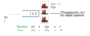
- Production systems also try to follow Dell Computer model, i.e. a combination of make-to-order and make-to-stock operations.
- Without the benefit of inventory, the process manager must keep sufficient capacity to process orders as they come in
Major Drivers of Performance:
The experiment in the previous slide shows that major drivers of performance in service systems are
- Capacity utilization
- Variability in (inter-)arrival times
- Variability in service times
Input characteristics:
- Arrival Process (inter-arrival time)
- Service Process (service time & no. of servers)
Output measures:
- Throughput and utilization
- Average waiting time in the queue and in the system
- Average numbers in the queue and in the system
Input Characteristics: Arrival Process
- Inter-arrival times are typically stochastic (random).
- Arrival rate (Ri): the average inflow rate of customer arrivals per unit of time.
- Average Inter-arrival time: the average time between two consecutive arrivals, which is equal to 1/Ri.
For example, if the arrival rate is 10 customer per min, then average inter-arrival time is 1/10 min or 6 sec.
For example, if the average inter-arrival time is 20 min, the arrival rate 1/20 per min or 3 per hour.
Input Characteristics: Service Process
- Processing times are typically stochastic.
- Service time Tp: the average processing time required to serve a customer.
- Unit service rate: the processing capacity of a server: 1/Tp
- Service rate Rp: the maximum rate at which customers can be processed by all c identical servers in a server pool: Rp = c/Tp .
For example, if Tp = 5 min, and there are 6 servers in the pool, the unit processing rate is 1/5 customers per min or 12 customers per hour, and service rate is 6/5 customer per min or 72 customer per hour.
Output Measures: Throughput and Utilization
Throughput: R = min(Ri,Rp ), utilization: u = R/Rp , safety capacity: Rs = Rp-R
- If Ri<r>p</r> → stable process
- If Ri>Rp → unstable process
- If Ri=Rp → only stable if there is no variability in arrival & service times.
For example with arrival rate of 10 customer per min, service time of 10 sec,
- With only one server (c=1), Rp = 6/min < Ri=10/min, so R=6/min, u=1, Rs=0 and system is unstable
- With two servers (c=2), Rp=12/min < Ri=10/min, so R=10/min, u=10/12=0.8, Rs=12-10=2/min and system is stable
What Else Utilization Represents?
Utilization is the fraction of server pool capacity that is busy serving customers.
Suppose Ri=10 per hour, and T p=0.5 hour. With 6 severs,
- Rp=6/0.5=12 per hour, R=min(10,12)=10 per hour so u=10/12=80% so 80% of the server pool capacity is busy serving customers.
- Also 10×0.5=5 hours of work comes to the system in every hour. Each server must provide 5/6 hour of service in each hour so will be busy in 5/6=80% of the time.
So utilization represents also the fraction of time each server is busy
Output Measures: Waiting Time and Queues
Assuming stability, R=Ri and
- Little’s law applied to servers: Ip= Ri*T<em>p</em> (average busy servers)
- Little’s law applied to the queue: Ii = Ri*Ti (average in queue)
- Little’s law applied to the whole process: I = Ri*T (average in system)
Performance Measures by Little’s Law
Note that out of four measures, Ii, Ti, I, T, we just need to know one as the other three are obtained using Little’s law.
- For instance, if we know I_i then
- Ti = Ii/Ri
- T = Ti+Tp
- I = T*Ri
Main Causes of Delays
High capacity utilization u = /iRR<strong>p</strong> , which is due to
- High arrival rate
- Low service rate Rp = c/T<em>p</em> , which might be due to small c and/or large Tp
High, unsynchronized, variability in
- Inter-arrival times
- Processing times
Measuring Variability:
- Variability in the inter-arrival time and processing time is measured using standard deviation (or Variance). Higher standard deviation (or Variance) means greater variability.
- Standard deviation is not enough to understand the extend of variability. Does a standard deviation of 20 for an average of 80 represents more variability than a standard deviation of 150 for an average of 1000?
- Coefficient of Variation: the ratio of the standard deviation to the mean, e.g. 20/80=0.25 and 150/1000=0.15 for above.
We use Ci for inter-arrival time and Cp for processing time
Flow Time- Utilization Curve:

Exponential Assumption:
The formula for Ii is only an approximation. It is only exact when c=1, and both inter-arrival and service times are exponentially distributed. Note that for exponential distribution coefficient of variation is one.
Performance Improvement Levers/Key Points:
- Decrease capacity utilization through
- Decreasing the arrival rate or increasing the unit processing rate
- Increasing the number of servers
- Decrease variability in inter-arrival and processing times
- Synchronize the available processing capacity with demand
