MMB-STATS-XO-digrams-etc Flashcards
(22 cards)
- X-O format:
R = ?
G = ?
X = ?
O = ?
R = random allocation to groups,
G = a non-random, naturally occurring group,
X = some environmental manipulation (level of IV or ‘treatment’),
O = an observation of a DV
- X-O format:
- Randomized two group designs a.k.a. randomised controlled trials a.k.a. posttest-only control group designs.
R > X1 – O1
R > X2 – O2
Participants are randomly allocated to two ‘treatment’ groups (often, treatment and control groups), and the DV is measured as the outcome variable. Note, O1 and O2 are measuring the same DV. A significant difference between the means (individual groups t-test) enables us to declare that the IV has an effect on the DV, as well as the direction of the effect.
Benefits: if properly done, guarantees internal validity. Drawbacks: may lack power compared with (2) below.
Analysed with independent groups t-test or (with multiple groups) one way ANOVA.
The IV, X, is a “between subjects” variable
3.
- Pretest-posttest control group designs a.k.a. before-after two group designs.
R > O1 – X1 – O2
R > O3 – X2 – O4
This has elements of both the post-test only and repeated measures designs (O1 – X1 – O2 on its own would be a very simple RM design).
Benefits: it has all the internal validity of the post-test only or RCT design, and it has the power of the latter, but avoids the threats to internal validity that would be involved in O1 – X1 – O2 by having a control condition, O3 – X2 – O4, which checks for effects of testing, history, maturation etc in the treatment group.
The IV, X, is a “between subjects” variable
4.
- Group Difference designs.
G1 > X – O1
G2 > X – O2
Participants are chosen according to membership in naturally occurring groups G1 and G2, and exposed to the same experimental intervention X, with the DV being measured as with the randomized two group design.
Note: for some purposes the group difference is the thing of interest in the study. For example, we may want to know whether people with autism differ from normal controls on some measure of empathy, or whether men and women differ in a visual-spatial task.
The IV, X, is a “between subjects” variable
5.
- Repeated measures designs.
a. Pretest-posttest design.
O1 – X – O2
This could also be written
X1 – O1 – X2 – O2 where the first X is the control condition (no treatment) and the second is the treatment condition. Therefore, it can be seen as the simplest kind of repeated measures design.
It could be analysed by using either RM ANOVA, or the paired samples t-test, or by calculating (O2 - O1) and testing whether it is significantly different from zero using the single sample t-test.
IV X is a “within subjects” variable
- (4. Repeated measures designs.)
b. Repeated measures design with time, and possibly treatment, as the variable.
O1 – X – O2 – X – O3 – X – O4 – X – O5 – ….
Usually analysed using a trend analysis in the repeated measures ANOVA program of SPSS. The result would be interpreted as showing a possible linear, quadratic etc trend of response to treatment over time.
IV X is a “within subjects” variable
- Repeated measures designs.
c. Repeated measures design with treatment levels as the variable.
Here some form of correction for carry-over effects is usually required.
With simple counterbalancing (only two levels of the IV):
R > X1 – O1 – X2 – O2
R > X2 – O3 – X1 – O4
Participants are randomly assigned to either the group experiencing X1 followed by X2, or the group given X2 first and then X1.
Analysed using RM ANOVA with the X variable as the RM variable. In this case a test for sphericity is needed.
If required to test for sequence and order effects, the group variable describing the counterbalancing factor should be included. Sequence effects are tested by significance of the group variable, and order effects by the group by RM variable interaction.
More complex variables with more than two levels are grouped according to a Latin square or equivalent method.
Multifactorial counterparts of these designs include two or more RM IVs, X, Y etc.
X it is a “within subjects” variable
- (5. Mixed designs.)
In which between subjects or group IVs, and repeated measures variables are entered into the analysis together. The groups may be either be drawn from the same population and randomly assigned to different experimenter manipulated environments, or may correspond to different naturally occurring groups such as gender.
R > O1 – XT – O2
R > O3 – XC – O4
And
R > XC – O1 – XT – O2
R > XT – O3 – XC – O4
The first one is essentially a between-groups comparison, in which the essential thing we are measuring is the difference in the DV between the first and second group.
The second one, having two groups is really a precaution against carry over effects – i.e. we are using counterbalancing – and the groups are not really “doing” anything of direct interest in the analysis.
There are both within subjects and between subjects variables.
9.
Assumptions in multiple regression: potential problems with distribution of error terms.
What are the 4 stages to check?
- Check for univariate and multivariate outliers in the IVs
- Get the plot of standardized residuals against predicted values of the DV
- Look for outliers in the solution
- Finally check that the residuals, ie the error terms, are distributed as they should be
10.
multiple regression: What does this plot show?
- Assumptions are met:
- Failure of normality:
- Non-liniarity:
- Heteroscedasticity:

Assumptions are met:
This is the ideal kind of plot
11.

multiple regression: What does this plot show?
Assumptions are met:
Failure of normality:
Non-liniarity:
Heteroscedasticity:
Failure of normality:

The error terms are skew upwards, so non-normal
12.

multiple regression: What does this plot show?
Assumptions are met:
Failure of normality:
Non-liniarity:
Heteroscedasticity:
Non-liniarity:

13.

multiple regression: What does this plot show?
Assumptions are met:
Failure of normality:
Non-liniarity:
Heteroscedasticity:
Heteroscedasticity:

the errors may be normally distributed but not with constant variance.
14.
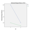
What does this line diagrams show?
- A possible ceiling effect
- a possible floor effect
- a scaling effect
- a qualatitive interaction

A possible ceiling effect

15.
What does this line diagrams show?
- a possible ceiling effect
- a possible floor effect
- a scaling effect
- a qualatitive interaction

a possible floor effect

16,
What does this line diagrams show?
- A possible ceiling effect
- a possible floor effect
- a scaling effect
- a qualatitive interaction

a scaling effect

The question you might ask, is how to tell whether this is more likely to be due to a scaling effect rather than a floor effect? The answer is that the values of the group means for level 1 of IV1 are 2 and 4, whereas for level 2 they are 4 and 8. The means are increasing in the same proportion for each group, namely they are doubling (from 2 to 4, and from 4 to 8). This suggests that the effect of IV1 is multiplicative rather than additive, but the multiplier is the same for both groups so it can be argued that the interaction is not genuine. In fact, for those who know about logs, a transformation of the IV by a logarithmic function would give two parallel lines, and the interaction would vanish.
17.
What does this line diagrams show?
- A possible ceiling effect
- a possible floor effect
- a scaling effect
- a qualatitive interaction

a qualatitive interaction
This is unquestionably a “real” interaction

- What is a categorical variable?
In statistics, a categorical variable is a variable that can take on one of a limited, and usually fixed, number of possible values, thus assigning each individual to a particular group or “category.”
- What is a continuous variable?
If a variable can take on any value between its minimum value and its maximum value, it is called a continuous variable; otherwise, it is called a discrete variable. Some examples will clarify the difference between discrete and continuous variables.
Continuous Variables would (literally) take forever to count. In fact, you would get to “forever” and never finish counting them. For example, take age. You can’t count “age”. Why not? Because it would literally take forever. For example, you could be:
25 years, 10 months, 2 days, 5 hours, 4 seconds, 4 milliseconds, 8 nanoseconds, 99 picosends…and so on. You couldturn age into a discrete variable and then you could count it. For example:
- Best way to tell if two categorical variables connected?
CHI squared test.

A chi-square statistic for two-way tables is sensitive to the strength of the observed relationship. The stronger the relationship, the larger the value of the chi-square test.
21.
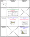
How would you display a continuous variable?
- BAR CHART: comparing between-group means: do they vary across groups? (use t-test, one way ANOVA)
- SCATTERPLOT: are two continuous variables connected? Outliers? (use Pearson’s bivariate correlation)

22.
Frequency measure -
HISTOGRAM: is a continuous variable normally distributed? Outliers? (use K-S test of normality)


