HBX- BA - 5 Flashcards

15%
The R2 value is approximately 0.15, or 15%. This means that 15% of the variation in selling price is explained by a home’s distance from Boston.
Multiple Regression (two or more independent variables) - Equation & Explanation
We use multiple regression to investigate the relationship between a dependent variable and multiple independent variables.
For multiple regression we rely less on scatter plots and more on numerical values and residual plots because visualizing three or more variables can be difficult.
Forecasting with a multiple regression equation is very similar to forecasting with a single variable linear model. However, instead of entering only one value for a single independent variable, we input a value for each of the independent variables.

Gross Relationship
The relationship between a single independent variable and a dependent variable. The gross relationship is affected by any variables that are related to the independent and/or dependent variable but are not included in the model.
In the graph below Because we are not considering any other factors
in this regression, we call this the gross effect of distance on price.
**We interpret the distance coefficient as meaning that
on average, prices decrease by $15,163 for each additional mile
a house is from Boston.

Net Relationship
A relationship between an independent variable and a dependent variable that controls for other independent variables in a multiple regression. Because we can never include every variable that is related to the independent and dependent variables, we generally consider the relationship between the independent & dependent variables to be net with regard to the other independent variables in the model, and gross with regard to variables that are not included.
CAN BE CALLED EITHER: net effect of distance on price or as the effect of distance on price controlling for house size.
The graph below tells us that for every additional mile a house is from Boston, on average price decreases by $10,840, assuming that the size of the house stays the same.

Multiple Regression Continued….
In Singular Regression - the variables being studied sometimes take on the effects of other variables. When they are separated in multiple regression, they’re able to be free and reflect their true values! (If we’ve included everything)
This also affects the equation (since there are so many variables) …
A coefficient is net with respect to all variables included in the model, but gross with respect to all omitted variables. It’s important to always keep in mind that included variables may be picking up the effects of omitted variables–
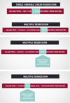
Which model would we use to predict the price of a house that is 2,700 square feet?
- SellingPrice=194,986.59+244.54(HouseSize)−10,840.04(distance from Boston)
- SellingPrice=13,490.45+255.36(HouseSize)
- SellingPrice=686,773.86–15,162.92(distance from Boston)
SellingPrice=13,490.45+255.36(HouseSize)
- Since we have data about just one independent variable, we should use a single variable regression model. This is a single variable linear regression model, in which house size is the only independent variable.
Suppose we want to forecast selling price based on house size and distance from Boston. Which equation should we use to forecast the price of a house that is 2,700 square feet and 15 miles from Boston?
- SellingPrice=194,986.59+244.54(HouseSize)–10,840.04(distance from Boston)
- SellingPrice=13,490.45+255.36(HouseSize)SellingPrice=13,490.45+255.36(HouseSize)
- SellingPrice=686,773.86–15,162.92(DistancefromBoston)
SellingPrice=194,986.59+244.54(HouseSize)–10,840.04(distance from Boston)
- Since we have data about two independent variables, house size and distance from Boston, we should use the multiple regression model with those two variables.

The expected selling price of a 2,700 square foot home that is 15 miles from Boston is B2+B3*2700+B4*15=$692,646.51. You must link directly to the values in order to obtain the correct answer.
Two houses are the same size, but located in different neighborhoods: House B is five miles farther from Boston than House A. If the selling price of House A was $450,000, what would we expect to be the selling price of House B?
SellingPrice=194,986.59+244.54(HouseSize)–10,840.04(DistancefromBoston)
SellingPrice=13,490.45+255.36(HouseSize)
SellingPrice=686,773.86–15,162.92(DistancefromBoston)
Approximately $396,000
Since the two houses are the same size, to predict the expected difference in selling prices we should use the net effect of distance on selling price (that is, the effect of distance on selling price controlling for house size). This value, -$10,840.04/mile, is found in the multiple regression model. House B is five miles farther from Boston than House A so House B’s expected selling price is: =House A’s selling price+net effect of distance on selling price≈$450,000–$10,840.04(5miles)≈$450,000–$54,200.20≈$395,799.80

Price
We are trying to estimate the price of the TV, so PricePrice is our dependent variable.

- 55
- 55 is the coefficient for PictureQualityPictureQuality.

The expected selling price of a 1,500 square foot home that is 10 miles from Boston is B15+B16*1,500+B17*10=$453,397.59. You must link directly to the values in order to obtain the correct answer.
Assume we have created two single linear regression models, and a multiple regression model to predict selling price based on House Size alone, Distance from Boston alone, or both. The three models are as follows, where House Size is in square feet and distance from Boston is in miles:
SellingPrice=13,490.45+255.36(HouseSize)
SellingPrice=686,773.86–15,162.92(distance from Boston)
SellingPrice=194,986.59+244.54(HouseSize)–10,840.04(distance from Boston)
House A and House B are the same size, but located in different neighborhoods: House B is five miles closer to Boston than House A. If the selling price of House A is $450,000, what would we expect to be the selling price of House B?
Approximately $504,000
Since the two houses are the same size, to predict the expected difference in selling prices we should use -$10,840.04/mile, the net effect of distance on selling price (that is, the effect of distance on selling price controlling for house size), which can be found in the multiple regression model. House B is five miles closer to Boston than House A so House B’s expected selling price is: House A’s selling price+net effect of distance on selling price ≈ $450,000+$10,840.04(5 miles) ≈ $450,000+$54,200.20 ≈ $504,200.20
In single variable regression, to measure the predictive power of a single independent variable we used R2 : the percentage of the variation in the dependent variable explained by the independent variable. For multiple regression models, we will rely on ______
Adjusted R2
Adjusted R2
A measure of the explanatory power of a regression analysis.
Adjusted R-squared = R-squared multiplied by an adjustment factor that decreases slightly as each independent variable is added to a regression model.
Unlike R-squared, which can never decrease when a new independent variable is added to a regression model, Adjusted R-squared drops when an independent variable is added that does not improve the model’s true explanatory power. Adjusted R2 should always be used when comparing the explanatory power of regression models that have different numbers of independent variables.
***R2 can only stay the same or increase. —> This is why we need Adjusted R2
In the case below, since the adjusted R-squared of the multiple regression
of price versus house size and distance is greater than the adjusted R-squared of either single variable regression, we can conclude that we gained real explanatory power by incorporating both independent variables
How should single variable regression models and multiple regression models be interpreted?
Recall that residuals represent the differences between the actual and predicted values of the dependent variable (selling price in this case).
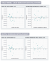
The house size residual plots for multiple and single variable linear regression represent different quantities:
- the residual plot for the single variable regression gives us insight into the gross relationship between price and house size;
- and the residual plot for multiple regression gives us insight into the net relationship between price and house size, controlling for distance.
The residual plots for the independent variable distance from Boston (the two plots on the right side in the panel) should be interpreted similarly:
- the residual plot for single variable regression gives us insight into the gross relationship between price and distance;
- and the residual plot for multiple regression gives insight into the net relationship between price and distance, controlling for house size.
P-Value + Multiple Regression
As in single variable linear regression, we must inspect the p-value of each independent variable to assess whether its relationship with the dependent variable is significant.
If the p-value is less than 0.05 for each of the independent variables, we can be 95% confident that the true coefficients of each of the independent variables are not zero. In other words, we can be confident that there is a significant linear relationship between the dependent variable and the independent variables.

Yes
Since the p-value for the independent variable (house size), 0.0000, is less than 0.05, we can be confident that the relationship between price and house size is significant. Recall that the p-value for the intercept does not determine the significance of the relationship between the dependent and independent variable, so even though the p-value for the intercept is greater than 0.05, we can still say that the relationship between price and house size is significant.

Yes
The p-values for the independent variables (house size and distance), 0.0000 and 0.0033, respectively, are less than 0.05, so we can be confident that the relationship between price, house size, and distance is significant.
What are the metrics to determine whether a multiple variable linear regression model is a good fit for our data.
1.)) Because R2 never decreases when independent variables are added to a regression, it is important to multiply it by an adjustment factor when we assess the fit of a multiple regression model. This adjustment factor compensates for the increase in R2 that results solely from increasing the number of independent variables.
-
Adjusted R2 is provided in the regression output.
It is particularly important to look at Adjusted R2, rather than R2, when comparing regression models with different numbers of independent variables.
2.)) In addition to analyzing Adjusted R2, we must test whether the relationship between the dependent variable and independents variables is linear and significant. We do this by analyzing the regression’s residual plots and the p-values associated with each independent variable’s coefficient.
- For multiple regression models, residual plots are an indispensable tool for detecting whether the linear model is a good fit.
- We rely heavily on residual plots for multiple regression models because the full relationship among multiple independent variables and the dependent variable is difficult or impossible to represent in a single scatter plot. (When there are two independent variables, the regression model describes the best fit plane through the data and the residuals can be seen on the three-dimensional scatter plot as well as on their individual residual plots.)
- The residuals are the difference between the historically observed values and the values predicted by the regression model.
- There is a residual plot for each independent variable included in the regression model.
- We can graph a residual plot for each independent variable to help detect patterns such as heteroskedasticity and nonlinearity.
- As with single variable regression models, if the underlying multiple relationship is linear, the residuals follow a normal distribution with a mean of zero and fixed variance.
- We should also analyze the p-values of the independent variables to determine whether there is a significant relationship between the variables in the model. If the p-value of each of the independent variables is less than 0.05, we conclude that there is sufficient evidence to say that we are 95% confident that there is a significant linear relationship between the dependent and independent variables.

Yes, this looks like a linear relationship.
There is nothing in this scatterplot to concern us.

No, there is heteroskedasticity.
There is evidence of heteroskedasticity; there is more variability at the lower values than at the higher values.
- Runs
- Strikeouts
- Completed Games
- ERA

The p-value column in the bottom table gives the significance level of each variable. The only p-values that are less than .05 are for the Intercept (which we do not assess for significance) and ERA. Thus, ERA is the only independent variable that is significant at p < .05. Note also that ERA is the only independent variable with a 95% confidence interval that does not contain 0.
Significant: ERA
Not significant: Runs, Strikeouts, Completed Games

- 0%
- 6298 or 63.0% is the R-square, which indicates how much variability is accounted for by the model.
Creating the Multiple Regression Output Table
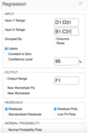
- Step 1- From the Data menu, select Data Analysis, then select Regression.
- Step 2- Enter the appropriate Input Y Range and Input X Range:
- The Input Y Range is the dependent variable, in this case selling price. The data are in column D with its label, D1:D31.
- The Input X Range should include both independent variables, in this case house size and distance from Boston. To ensure that the independent variables are labeled correctly in the output table, enter the data with its labels in column B and column C, B1:C31.
- Note that to run a regression in Excel the independent variables must be in contiguous columns. (sharing a common border)
- Since we included the cells containing the variables’ labels when inputting the ranges, check the Labels box.
- Step 3 - Scroll down and make sure to check the Residuals and Residual Plots boxes to ensure we see the relevant residual information. You will not be able to submit if you do not include the residual plots.
REGRESSION STATISTICS TABLE: Multiple R

REGRESSION STATISTICS TABLE: Standard Error

REGRESSION STATISTICS TABLE: Observations

ANOVA TABLE: df, residual, regression, total df
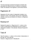
ANOVA TABLE: SS, Regression, Residual, Total

ANOVA TABLE: MS

ANOVA TABLE: F & Significance F

REGRESSION COEFFICIENTS TABLE: Coefficients & Standard error

REGRESSION COEFFICIENTS TABLE: T-Stat & P-Value

REGRESSION COEFFICIENTS TABLE: Lower/Upper 95% & Residual Output
- Year and Quarter
- Housing Starts (thousands)
- House Price Index
- Unemployment Rate
- Disposable Income
- Home Owner Vacancy Rates

- House Price Index
- Unemployment Rate
- Disposable Income
- Home Owner Vacancy Rates
House Price Index, Unemployment Rate, Disposable Income, and Home Owner Vacancy Rates are the independent variables used to create the regression model.
Housing Starts (thousands) is the dependent variable used to create the regression model.
Year and Quarter is not included as a dependent or independent variable.

Input Y Range: B1:B81
Input X Range: C1:F81

3
There are three independent variables included in the model: cylinders, engine displacement, and passenger volume. The three independent variables are selected from the specified attributes we wish to include. Make and model variables are not included as independent variables for this multiple regression model.

Input Y Range: F1:F59
Input X Range: C1:E59
Multicollinearity
Multicollinearity occurs when two independent variables are so highly correlated that it is difficult for the regression model to separate the effect each variable has on the dependent variable.
Multicollinearity can obscure the results of a regression analysis. If adding a new independent variable decreases the significance of another independent variable in the model that was previously significant, multicollinearity may well be the culprit. Another symptom of multicollinearity is when the R-square of a regression is high but none of the independent variables are significant.
If a variable that was significant becomes insignificant when we add it to a regression model, we can usually attribute it to a relationship between two or more of the independent variables.
(you can check this significance with the p-value)
One way to detect multicollinearity is by checking to see if any variable’s P value increases when a new independent variable is added.
- If we’re using the regression model to make predictions, multicollinearity is usually not a problem, so we might keep the lot size variable in the model. It improves the adjusted R-squared, and more importantly, our managerial judgment tells us that lot size should have an impact on price that is separate from the effect of house size.
- If we’re trying to understand the net effects of the independent variables, then multicollinearity is a problem that should be addressed.
The best way to reduce multicollinearity is simply to increase the sample size. More observations may help discern the net effects of the individual independent variables. We can also reduce or eliminate multicollinearity by removing one of the collinear independent variables. Doing this requires careful analysis of the relationships among the variables.

Dummy Variables
=IF(logical_test, [value_if_true], [value_if_false])
Steps below using an example from the module!
- Step 1
- In cell C2, enter the function =IF(B2=”Monday”,1,0).
- This function says that if cell B2 equals “Monday”, then enter a 1 in cell C2 and if cell B2 does not equal “Monday”, then enter a 0 in cell C2.
- You can also enter =IF(B2=$C$1,1,0) since cell C1 equals Monday. Note that you must lock cell C1 so that when you copy the function, it continues to reference C1.
- Step 2
- Copy and paste the formula from cell C2 into cells C3:C32.
- This assigns a dummy variable value in column C for each data point in column B.
- To use auto-fill, enter the first value in cell C2. Highlight C2 and place your cursor at the bottom right-hand corner of the cell. The cursor will turn into a black cross. Drag the cross down the column until you reach cell C32. When you release the mouse, the values will auto-fill.

base case
base case- The category of a categorical variable for which a dummy variable is NOT included in a regression model. A regression model with a categorical variable that has n categories should have n-1 dummy variables. The coefficients of the dummy variables included in the regression model are interpreted in relation to the base case. The analyst can select any category to be excluded from the regression model; however, different base cases lead to different interpretations of the dummy variables’ coefficients.
For example, suppose we are trying to determine the average difference in height between men and women in a sample, and suppose that on average men are 5 inches taller than women in the sample. If we use Female as the base case then the coefficient for the dummy variable for Male would be +5. If we use Male as the base case, the coefficient for the dummy variable for Female would be -5.

Suppose we want to assign dummy variables to months (Jan-Dec) and day of week (Sun-Sat). How many dummy variables do we need?
17
For each category, we must use one fewer dummy variables than the number of options for that category. Since month and day of week are separate categories, we should subtract one for each category. Thus we would use 12–1=11 variables for month and 7–1=6 variables for day of week, giving a total of 17 dummy variables
Suppose we want to assign dummy variables to months (Jan-Dec). How many dummy variables do we need?
11

Sales=−631,085+533,024(Red)+50.5(Advertising)
We always interpret the coefficient of a dummy variable as being the expected change in the dependent variable when that dummy variable equals one compared to the base case. In this case, controlling for advertising, we expect sales for red sneakers to be $533,024 more than blue sneakers. It is helpful to view this model graphically. Consider two parallel regression lines: one for red sneakers and one for blue sneakers. The vertical distance between the lines is the average increase in sales the manager can expect when red sneakers are sold versus blue sneakers, controlling for advertising. The slope of the two lines, 50.5, is the same: It tells us the average increase in sales, controlling for sneaker color, as we increase advertising by $1.
lagged variable
A type of independent variable often used in a regression analysis. When data are collected as a time series, a regression analysis is often performed by analyzing values of the dependent with independent variables from the same time period. However, if researchers hypothesize that there is a relationship between the dependent variable and values of an independent variable from a previous time period, may include a “lagged variable”, that is, and independent variable based on data from a previous time period.
Advertising provides a good example, because its effects often persist.
For**example: last year’s advertising may still influence this year’s sneaker sales. We can incorporate the delayed effect of an independent variable on the dependent variable using a lagged variable.
Spreadsheet: Let’s walk through how to create a lagged variable.
Sales=−631,085+533,024(Red)+50.5(Advertising)
- Step 1: Copy the advertising data in range C2:C11.
- Step 2: To create the lagged variable, paste the advertising data into the range D3:D12 in Column D, under the title “Previous Year’s Advertising.” That is, the value from C2 will be pasted into D3, from C3 into D4, and so on until the value in C11 is pasted into D12. For example, in D3, the value for 2005 Previous Year’s Advertising will be the advertising expenditure for 2004, $35,000.
- When completed properly, Row 12 should contain only one observation (in D12). Since we do not have advertising data for 2003, we do not know Previous Year’s Advertising for 2004; thus, D2 should be blank.
- Note: Rather than copying and pasting, you may also choose to link directly to cells (for example, cell D3 would contain the formula =C2).
Points-
- The first row has all the necessary data except a lagged value.
- And the last row has only a lagged value.
- Since every observation we use needs a value for each variable, we must remove both the first observation and the newly added row.
- Thus, by introducing a lagged variable, we lose one data point. We run and interpret a regression with lagged variables as we would any other multiple regression model.
We also need to think carefully about what the appropriate lag time should be. How long do we think the effects of an advertising campaign would last? A month, six months, a year?Since we have only annual data, we can only analyze effects in yearly increments. For example, if we believe that the effects last two years, we can include an additional variable with a two-year lag. We have to be careful though. Remember that each additional lagged variable reduces the number of observations we can use, and hence may reduce accuracy and explanatory power.
Adding a lagged variable is costly in two ways:
- Each lagged variable creates an incomplete line of data. If we have a single lagged variable, our first observation will be incomplete. If we have two lagged variables, our first two observations will be incomplete, and so on. The loss of each data point decreases our sample size by one, which reduces the precision of our estimates of the regression coefficients.
- In addition, if the lagged variable, or variables, do not increase the model’s explanatory power, the addition of the variable decreases Adjusted R2, just as the addition of any variable to a regression model can.
We include lagged variables only if we believe the benefits of doing so outweigh the loss of one or more observations and the “penalty” imposed by the adjustment to R2. Despite those costs, lagged variables can be very useful. Because they pertain to previous time periods, they are usually available ahead of time. They are often good leading indicators, which help us predict future values of a dependent variable.

create a regression model with Lagged Data
Reducing the number of usable rows means that the labels are no longer contiguous with the data of interest, so you should leave the Labels box unchecked.
Note that NOT checking the Labels box is unique to this data setup (when the lagged data has created blank cells between the number values and the column labels). Generally, you would always want to use labels in a regression.
- Step 1: Select Data, then Data Analysis, then Regression.
- Step 2: Enter your Input Y range as B3:B11. (Notice that we cannot use the data for Sales in B2 since we do not have an entry for D2)
- Step 3: Enter your Input X range as C3:D11. (Notice that we cannot use the data for Advertising for 2004 in C2 since we do not have an entry for D2. Moreover, we cannot use the data in D12 since we don’t have data for other variables for 2014.)
- Step 4: Check the Residuals and Residual Plot boxes, but DO NOT check the Labels box. Click OK to start the regression analysis.

We may be able to reduce multicollinearity by either________ or ________
We may be able to reduce multicollinearity by either increasing the sample size or removing one (or more) of the collinear variables.
Review the sections at the end of each BA - Real Examples <3
DO IT- THIS STAYS PURPLE UNTIL YOU DO SO


