COMP-311 Final Flashcards
(73 cards)
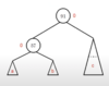
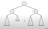
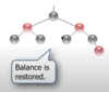
2-3 Trees
- 1 to 2 values in each node
- 0 to 3 links to other nodes
- Balanced, non-binary trees
- All leaves are at the lowest level
Approximately, what is the maximum height of a binary search tree of N nodes?
log2 n
The following items are inserted into a B-tree: 3, 6, 5, 2, 4, 7, 1. Which node is the deepest?
Question doesn’t make sense. Must specify the degree of the B-Tree. Even then, all leaves are at the bottom so there will be many nodes at the “deepest” level.
The following items are inserted into a 2-3 tree: 3, 6, 5, 2, 4, 7, 1. Which node is the deepest?
3, 5
1, 2 | 4 | 6, 7
What operation(s) will require the most time in a balanced binary search tree?
Insertion and deletion have to perform rotations, so they will take longer than search, but they’re all still O(log n).
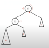
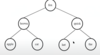
Show the 2-3 tree after inserting each of the following values one at a time: 1, 4, 9
7
3 | 11
7
1, 3 | 11
3, 7
1 | 4 | 11
3, 7
1 | 4 | 9, 11
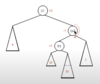
2-3 Tree Insertion Algorithm
- Find the leaf where the item should be inserted
- If there is only 1 other item in the leaf, put the new item in the leaf
- Otherwise, split the node into two other nodes with the leftmost and rightmost elements, ejecting the middle element up to the parent node.
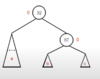
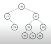
Show the following tree after inserting each of the following one at a time: 9, 13, 17
7
3 | 11, 15
7, 11
3 | 9 | 15
7, 11
3 | 9 | 13, 15
11
7 | 15
3 | 9 || 13 | 17
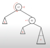
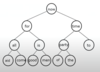
Show the 2-3 tree that would be built for the following sentence: “Rather fail with honor than succeed by fraud.”
rather
fail, rather
rather
fail | with
rather
fail, honor | with
rather
fail, honor | than, with
rather, than
fail, honor | succeed | with
rather
fail | than
by | honor || succeed | with
rather
fail | than
by | fraud, honor || succeed | with
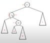
2-3-4 Trees
- Like 2-3 trees, but with another data element and reference
- Node can hold 1-3 data elements
- Node can hold 0-4 references
- Split full nodes upon descent for insertion - ensures that there is always space in a leaf to insert the new item
2-3-4 Trees continued
- 2-3-4 trees are equivalent to Red-Black trees
- 2-node is a black node
- 4-node is a black node with 2 red children
- 3- node is a black node with a read left child or a black node with a red right child (arbitrary choice)
B-Trees
- The natural extension to 2-3-4 trees
- A node holds n data elements and n+1 references to other nodes
- Said to be of degree n
- Algorithms work the same as on 2-3-4 trees
B-Tree Uses
- Disk structures large databases and indexes
- Very high order (200 or more) leads to wide but shallow trees
- Still need to do many comparisons within a node to locate which reference to follow
Selection Sort Algorithm
- Divide array into left (sorted) and right (unsorted) sections
- Find smallest element in the right section
- Swap smallest into first right-side index
- O(n2)
Insertion Sort Algorithm
- Divide array into left (sorted) and right (unsorted) sections
- Pick next element in right section
- Find where it fits in the left section
- O(n2)
Bubble Sort Algorithm
- So long as an exchange takes place
- Loop over all the elements pairwise
- If the elements are out of order, then exchange them
Show the progress of each pass of the selection sort for the following array. How many passes are needed? How many comparisons are performed? How many exchanges?
Original
40 | 35 | 80 | 75 | 60 | 90 | 70 | 75
- # passes: 7 (i.e. n-1)
- # comparisons: 28 (i.e. n * (n-1)/2)
- # exchanges: 7 (i.e. n-1)
Pass1
35 | 40 | 80 | 75 | 60 | 90 | 70 | 75
Pass 2
35 | 40 | 80 | 75 | 60 | 90 | 70 | 75
Pass 3
35 | 40 | 60 | 75 | 80 | 90 | 70 | 75
Pass 4
35 | 40 | 60 | 70 | 80 | 90 | 75 | 75
Pass 5
35 | 40 | 60 | 70 | 75 | 90 | 80 | 75
Pass 6
35 | 40 | 60 | 70 | 75 | 75 | 80 | 90
Pass 7
35 | 40 | 60 | 70 | 75 | 75 | 80 | 90
Show the progress of each pass of the bubble sort for the following array. How many passes are needed? How many comparisons are performed? How many exchanges?
Original
40 | 35 | 80 | 75 | 60 | 90 | 70 | 75
- # passes: 4 (varies)
- # comparisons: 22 (varies 7+6+5+4)
- # exchanges: 9 (varies)
Pass 1
35 | 40 | 75 | 60 | 80 | 70 | 75 | 90
Pass 2
35 | 40 | 60 | 75 | 70 | 75 | 80 | 90
Pass 3
35 | 40 | 60 | 70 | 75 | 75 | 80 | 90
Pass 4
35 | 40 | 60 | 70 | 75 | 75 | 80 | 90
Show the progress of each pass of the insertion sort for the following array. How many passes are needed? How many comparisons are performed? How many shifts?
Original
40 | 35 | 80 | 75 | 60 | 90 | 70 | 75
- # passes: 7 (i.e. n-1)
- # comparisons: 15 (varies)
- # exchanges: 13 (varies)
Pass 1
35 | 40 | 80 | 75 | 60 | 90 | 70 | 75
Pass 2
35 | 40 | 80 | 75 | 60 | 90 | 70 | 75
Pass 3
35 | 40 | 75 | 80 | 60 | 90 | 70 | 75
Pass 4
35 | 40 | 60 | 75 | 80 | 90 | 70 | 75
Pass 5
35 | 40 | 60 | 75 | 80 | 90 | 70 | 75
Pass 6
35 | 40 | 60 | 70 | 75 | 80 | 90 | 75
Pass 7
35 | 40 | 60 | 70 | 75 | 75 | 80 | 90
Shell Sort Algorithm
- A better insertion sort
- Sorts parallel sub-arrays
- Decreases gap, and sort larger arrays each pass
- Proven O(n(3/2)) for gaps from 2k-1
- Probably O(n(5/4)) or even O(n(7/6)) for initial gap of n/2, then subsequent gaps dividing by 2.2
Heap Sort Algorithm
- Naive algorithm
- Insert values into a heap
- Repeatedly extract-max
- Can be done efficiently in-place
- Convert array to heap
- For each element: Swap max with last element, Reconvert to a heap
Tree sort algorithm
- Insert values into a binary search tree
- Perform in-order traversal to get sorted list
Merge Sort Algorithm
- “Divide and conquer” algorithm
- Splits list in two
- Sort sub-lists (recursively)
- Merge sub-lists
Quick Sort Algorithm
- “Divide and conquer” algorithm
- Select pivot
- Partition list into:
- items less than pivot
- pivot
- items greater than pivot
- Sort the items on either side of the pivot (recursively)