Chapter 7: Pruning in Decision Trees Data Preparation

Question 1

Decision Tree Algorithms

Answer 1

• At each node, available attributes are evaluated on the basis of separating the classes of the training examples.
• A goodness function is used for this purpose.
• Typical goodness functions:
  
  • information gain (ID3/C4.5)
  • information gain ratio
  • gini index (CART)

Question 2

Computing Information

Answer 2

• Information is measured in bits
  
  • Given a probability distribution, the info required to predict an event, i.e. if play is yes or no, is the distribution’s entropy
  • Entropy gives the information required in bits (this can involve fractions of bits!)
• Formula for computing the entropy:
  
  • entropy(p₁…p_n) = - p₁ logp₁ -…- _np logp_n

Question 3

Industrial-Strength Algorithms

Answer 3

• For an algorithm to be useful in a wide range of real- world applications it must:
  
  • Permit numeric attributes
  • Allow missing values
  • Be robust in the presence of noise
• Basic schemes need to be extended to fulfill these requirements

Question 4

Pruning

Answer 4

•  Prepruning tries to decide a priori when to stop creating subtrees
  
  • Halt construction of decision tree early
  • Use same measure as in determining attributes, e.g., halt if InfoGain < threshold
  • Most frequent class becomes the leaf node
  • This turns out to be fairly difficult to do well in practice
    
    • due to “combination-lock effect”, i.e. two attributes individually have nothing to contribute but are powerful predictors when combined
• Postpruning simplifies an existing decision tree
  
  • Construct complete decision tree
  • Then prune it back
  • Used in C4.5, CART
  • Needs more runtime than prepruning

Question 5

Postpruning

Answer 5

Subtree replacement replaces a subtree with a single leaf node (main method).

Subtree raising moves a subtree to a higher level in the decision tree, subsuming its parent

Question 6

When to Prune a Tree?

Answer 6

• To determine if a node should be replaced, compare the error rate estimate for the node with the combined error rates of the children.
• Replace the node if its error rate is less than combined rates of its children.
• Prune only if it reduces the estimated error
  • Error on the training data is NOT a useful estimator
• Use a hold-out set for pruning (“reduced-error pruning”)
  
  • Limits data you can use for training
• C4.5’s method
  
  • Derive confidence interval from training data
  • Use a heuristic limit for the error rate, derived from the confidence interval for pruning
  • Shaky statistical assumptions (because it is based on training data), but works well in practice

Question 7

Bernoulli Process

Answer 7

•  The Bernulli process is a discrete-time stochastic process consisting of a sequence of independent random variables (i.e., a sequence of Bernulli trials)
•  Applied to situations where an event does either occur (success) or not occur (failure)
  
  • Let the probability of occurrences be 𝑝, the probability of no occurrence be 𝑞 = 1 − 𝑝.
  • Let the total number of independent trials be 𝑛, and the number of successes be 𝑘.
•  The probability of 𝑘 successes in n trials is the probability mass function (pmf) of the Binomial Distribution B:

Question 8

Central Limit Theorem Revisited

Answer 8

• The central limit theorem states that the standardized average of any population of i.i.d. random variables 𝑋𝑖 with mean 𝜇_𝑋 and variance 𝜎² is asymptotically ~𝑁(0,1), or
• Asymptotic Normality implies that 𝑃(𝑍 < 𝑧 )–>  Φ(𝑧) a - n -> infinity, 𝑜𝑟 𝑃(𝑍 < 𝑧) equal  Φ(𝑧)

Question 9

Using the Confidence Interval of a Normal Distribution

Answer 9

• C4.5 uses a heuristic limit for the error rate, derived from the confidence interval of the error rate for pruning
•  𝑥% confidence interval [– 𝑧<=  𝑋<=  𝑧] for random variable with 0 mean is given by: Pr[-z
•  With a symmetric distribution:
• Pr[z <= <=X  z]=1-2xPr[X >= z]

Question 10

Confidence Limits

Answer 10

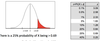
• Confidence limits c for the standard normal distribution with 0 mean and a variance of 1:
• There is a 25% probability of X being > 0.69 Pr[0.69  X  0.69]
• To use this we have to reduce our random variable f to have 0 mean and unit variance

Question 11

Transforming f

Answer 11

•  You prune the tree stronger
  
  • If c goes down=>z goes up and also p goes up
  • If n goes down=>p goes up 
  • with p as an estimator for the error rate

Question 12

C4.5’s Method

Answer 12

•  Error estimate e for a node (:= upper bound of confidence interval):
  
  • see pic
  • If c = 25% then z = 0.69 (from normal distribution)
  • f is the error on the training data 
  • n is the number of instances covered by the node
• Even if information gain increases, e might increase as well
• Error estimate for subtree is weighted sum of error estimates for all its leaves

Question 13

C4.5 Example

Answer 13

Question 14

From Trees to Rules

Answer 14

• Simple way: one rule for each leaf
  
  • Often these rules are more complex than necessary
• C4.5rules:
  
  • greedily prune conditions from each rule if this reduces its estimated error (as discussed above)
• Then
  
  • look at each class in turn
  • consider the rules for that class
  • find a “good” subset (guided by Occam’s Razor)
  • Finally, remove rules (greedily) if this decreases error on the training data

Question 15

C4.5 and C4.5rules: Summary

Answer 15

• C4.5 decision tree algorithm has two important parameters
  
  • Confidence value (default 25%): lower values incur heavier pruning
  • Minimum number of instances in the two most popular branches (default 2)
• Classification rules
  
  • C4.5rules slow for large and noisy datasets
  • Commercial version C5.0rules uses a different pruning technique
    
    • Much faster and a bit more accurate

Question 16

Knowledge Discovery Process

Answer 16

Question 17

Data Understanding: Quantity

Answer 17

• Number of instances (records)
  
  • Rule of thumb: 5,000 or more desired (nice to have)
  • if less, results are less reliable; use special methods (boosting, …)
• Number of attributes
  
  • Rule of thumb: Start out with less than 50 attributes
  • If many attributes, use attribute selection
• Number of targets
  
  • Rule of thumb: >100 for each class
  • if very unbalanced, use stratified sampling

Question 18

Data Understanding

Answer 18

• Visualization
• Data summaries
  
  • Attribute means
  • Attribute variation
  • Attribute relationships

Question 19

Data Cleaning: Outline

Answer 19

• Convert data to a standard format (e.g., arff or csv)
• Unified date format
• Missing values
• Fix errors and outliers
• Convert nominal fields whose values have order to numeric
• Binning (i.e. discretization) of numeric data

Question 20

Data Cleaning: Missing Values

Answer 20

• Missing data can appear in several forms:
  
  • “0” “.” “999” “NA” …
• Standardize missing value code(s) Dealing with missing values:
  
  • Ignore records with missing values
  • Treat missing value as a separate value
  • Imputation: fill in with mean or median values

Question 21

Conversion: Ordered to Numeric

Answer 21

• Ordered attributes (e.g. Grade) can be converted to numbers preserving natural order, e.g.
  
  • A 4.0
  • A- 3.7
  • B+3.3
  • B 3.0
• Why is it important to preserve natural order?
  
  • To allow meaningful comparisons, e.g. Grade > 3.5

Question 22

Conversion: Nominal, Few Values

Answer 22

• Multi-valued, unordered attributes with small no. of values
  
  • e.g. Color=Red, Orange, Yellow, …
  • for each value v create a binary “flag” variable C_v , which is 1 if Color=v, 0 otherwise

Nominal, many values: Ignore ID-like fields whose values are unique for each record

Question 23

Data Cleaning: Discretization

Answer 23

• Discretization reduces the number of values for a continuous attribute
• Why?
  
  • Some methods can only use nominal data
    
    • E.g., in ID3, Apriori, most versions of Naïve Bayes, CHAID
  • Helpful if data needs to be sorted frequently (e.g., when constructing a decision tree)
  • Some methods that handle numerical attributes assume normal distribution which is not always appropriate
• Discretization is useful for generating a summary of data
• Also called “binning”

Question 24

Discretization: Equal-Width

Answer 24

Question 25

Discretization: Equal-Width May Produce Clumping

Answer 25

Question 26

Discretization: Equal-Frequency

Answer 26

Question 27

Discretization: Class Dependent (Supervised Discretization)

Answer 27

•  Treating numerical attributes as nominal discards the potentially valuable ordering information
•  Alternative: Transform the 𝑘 nominal values to 𝑘 − 1 binary attributes. The (𝑖 − 1)-th binary attribute indicates whether the discretized attribute is less than 𝑖

Question 28

Discretization Considerations

Answer 28

• Equal Width is simplest, good for many classes
  
  • can fail miserably for unequal distributions
• Equal Frequency gives better results
  
  • In practice, “almost-equal” height binning is used which avoids clumping and gives more intuitive breakpoints
  • Also used for clustering (when there is no “class”)
• Class-dependent can be better for classification
  
  • Decision trees build discretization on the fly
  • Naïve Bayes requires initial discretization
• Other methods exist …

Question 29

Unbalanced Target Distribution

Answer 29

• Sometimes, classes have very unequal frequency
  
  • Churn prediction: 97% stay, 3% churn (in a month)
  • Medical diagnosis: 90% healthy, 10% disease
  • eCommerce: 99% don’t buy, 1% buy
  • Security: >99.99% of Germans are not terrorists
• Similar situation with multiple classes
• Majority class classifier can be 97% correct, but useless

Question 30

Building Balanced Train Sets

Answer 30

Question 31

Attribute Selection

Answer 31

• Aka feature / variable / field selection
• If there are too many attributes, select a subset that is most relevant.
• Remove redundant and/or irrelevant attributes
  
  • Rule of thumb – keep top 50 attributes

Question 32

Reasons for Attribute Selection

Answer 32

• Simpler model
  
  • More transparent
  • Easier to interpret
• Faster model induction
  
  • What about overall time?
• What about the accuracy?
  
  • The addition of irrelevant attributes can negatively impact the performance of kNN, DT, regressions, clustering, etc.
    
    • Experiments: Adding a random attribute to a DT learner can decrease the accuracy by 5-10% (Witten & Frank, 2005)
    • Instance-based methods are particularly weak in the presence of irrelevant attributes (compared with only a few instances)

Question 33

Attribute Selection Heuristics

Answer 33

• Stepwise forward selection
  
  • Start with empty attribute set
  • Add “best” of attributes (e.g. using entropy)
  • Add “best” of remaining attributes
  • Repeat. Take the top n (a certain threshold value)
• Stepwise backward selection
  
  • Start with entire attribute set
  • Remove “worst” of attributes
  • Repeat until n are left.

Question 34

Attribute Selection

Answer 34

• Using entropy for attribute selection
  
  • Calculate information gain of each attribute
  • Select the n attributes with the highest information gain
• Experiences
  
  • Lead to local, not necessarily global optima
  • Nevertheless, they perform reasonably well
  • Backward selection performed better than forward selection
  • Forward selection leads to smaller attribute sets and easier models
• Attribute selection is actually a search problem
  • Want to select subset of attributes giving most accurate model

Question 35

Basic Approaches to Attribute Selection

Answer 35

• Remove attributes with no or little variability
  
  • Examine the number of distinct attribute values
  • Rule of thumb: remove a field where almost all values are the same (e.g. null), except possibly in minp % or less of all records.
• Remove false predictors (“leakers”)
  
  • False predictors are fields correlated to target behavior, which describe events that happen at the same time or after
  • E.g. student final grade, for the task of predicting whether the student passed the course

Question 36

Text Mining

Answer 36

• Many text databases exist in practice
  
  • News articles
  • Research papers
  • Books
  • Digital libraries
  • E-mail messages
  • Web pages

Question 37

Text Mining Process

Answer 37

• Text preprocessing
  
  • Syntactic/Semantic text analysis
• Features Generation
  
  • Bag of words
• Features Selection
  
  • Simple counting
  • Statistics
•  Text/Data Mining
  
  • Classification of documents
  • Clustering of documents
•  Analyzing result

Question 38

Text Attributes

Answer 38

• For each word, generate a boolean attribute indicating whether the text of the instance contains the word
  
  • Alternatively, the attribute may indicate the number of the word’s occurrences
  • If “too many” words, keep only the more frequent ones
  • Stemming algorithms reduce words to their root, e.g. guarantee, guaranteeing, guaranteed

Question 39

Data Mining: Technical Memo Example: Titles

• c1 Human machine interface for Lab ABC computer applications
• c2 A survey of user opinion of computer system response time
• c3 The EPS user interface management system
• c4 System and human system engineering testing of EPS
• c5 Relation of user-perceived response time to error measurement
• m1 The generation of random, binary, unordered trees
• m2 The intersection graph of paths in trees
• m3 Graph minors IV: Widths of trees and well-quasi-ordering
• m4 Graph minors: A survey

Answer 39

Question 40

Data mining: “Search” versus “Discover”

Answer 40