Chapter 6: Decision Trees

Question 1

Decision Trees

Answer 1

• An internal node is a test on an attribute.
• A branch represents an outcome of the test, e.g., Color=red.
• A leaf node represents a class label or class label distribution.
• At each node, one attribute is chosen to split training examples into distinct classes as much as possible.
• A new case is classified by following a matching path to a leaf node

Question 2

Building Decision Tree

Answer 2

• Top-down tree construction (Recursive Algo ⇒ End up with huge tree. If model is over fitted means it does not generalize well )
  
  • At start, all training examples are at the root.
  • Partition the examples recursively by choosing one attribute each time.
• Bottom-up tree pruning
  
  • Remove subtrees or branches, in a bottom-up manner, to improve the estimated accuracy on new cases

Question 3

Choosing the Splitting Attribute

Answer 3

• At each node, available attributes are evaluated on the basis of separating the classes of the training examples.
• A “goodness” function is used for this purpose. Typical goodness functions:
  
  • information gain (ID3/C4.5)
  • information gain ratio
  • gini index (CART)
• Pcrkct split criteria: Splits data in two sides - Yes and No. ⇒ clean subnodes

Question 4

A Criterion for Attribute Selection

Answer 4

• Which is the best attribute?
  
  • The one which will result in the smallest tree
  • Heuristic: choose the attribute that produces the “purest” nodes
• Popular impurity criterion: information gain
  
  • Information gain increases with the average purity of the subsets that an attribute produces
• Strategy: choose attribute that results in greatest information gain

Question 5

Computing Information

Answer 5

• Information is measured in bits
  
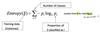
  • Given a probability distribution, the info required to predict an event, i.e. if play is yes or no, is the distribution’s entropy
  • Entropy gives the information required in bits (this can involve fractions of bits!)
• Formula for computing the information entropy:
  
  • Defines how ordered a system is

Question 6

Example: attribute “Outlook”

Answer 6

Question 7

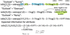
Computing the Information Gain

Answer 7

Question 8

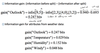
Continuing to Split

Answer 8

Question 9

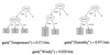
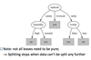
The Final Decision Tree

Answer 9

Question 10

Wish List for a Purity Measure

Answer 10

• Properties we require from a purity measure:
  
  • When node is pure, measure should be zero (=0)
  • When impurity is maximal (i.e. all classes equally likely), measure should be maximal (e.g., 1 for boolean values)
  • Multistage property: Info[2,3,4]=Info[2,7]+7/9 Info[3,4]
• Entropy is a function that satisfies these properties

Question 11

Entropy

Answer 11

• Entropy in general, describes the randomness of a system
  
  • Entropy = 0 describes a perfectly ordered system
• The term was used in thermodynamics and and statistical mechanics „ A Mathematical Theory of Communication“ by Claude Shannon 1948 defines entropy and information theory
  
  • „uncertainty about the contents of a message“

Question 12

Expected Information Gain

Answer 12

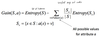
Gain(S,a) is the information gained adding a sub-tree (Reduction in number of bits needed to classify an instance)

Problems?

Question 13

Highly-Branching Attributes

Answer 13

• Problematic: attributes with a large number of values (extreme case: ID code) Subsets are more likely to be pure if there is a large number of values
  
  • Information gain is biased towards choosing attributes with a large number of values
  • This may result in overfitting (selection of an attribute that is non-optimal for prediction)

Question 14

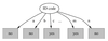
Split for ID Code Attribute

Answer 14

Entropy of split = 0 (since each leaf node is “pure”), having only one case. Information gain is maximal for ID code

Question 15

Gain Ratio

Answer 15

• Gain ratio: a modification of the information gain that reduces its bias on high-branch attributes 4 ->Corrects ID problem
• Gain ratio takes number and size of branches into account when choosing an attribute
• It corrects the information gain by taking the intrinsic information of a split into account (i.e. how much info do we need to tell which branch an instance belongs to)

Question 16

Computing the Gain Ratio

Answer 16

Example: intrinsic information for ID code

intrinsic_info(1,1, ,1) = 14 x( - 1/14 x log1/14)= 3.807 bits Importance of attribute decreases as intrinsic information grows.

Question 17

More on the Gain Ratio

Answer 17

• „Outlook” still comes out top
• However:
  
  • “ID code” has still greater gain ratio (0.246)
  • Standard fix: ad hoc test to prevent splitting on that type of attribute
• Problem with gain ratio: it may overcompensate
  
  • May choose an attribute just because its intrinsic information is very low
  • Standard fix:
    
    • First, only consider attributes with greater than average information gain
    • Then, compare them on gain ratio

Question 18

The Splitting Criterion in CART

Answer 18

• Classification and Regression Tree (CART)
• Developed 1974-1984 by 4 statistics professors
  
  • Leo Breiman (Berkeley), Jerry Friedman (Stanford), Charles Stone (Berkeley), Richard Olshen (Stanford)
• Gini Index is used as a splitting criterion
• Both C4.5 and CART are robust tools
• No method is always superior – experiment!

Question 19

Gini Index for 2 Attribute Values

Answer 19

• For example, two classes, Pos(itive) and Neg(ative), and dataset S with p Pos-elements and n Neg-elements.
  
  • fp = p / (p+n)
  • fn = n / (p+n)
  • Gini(S) = 1 – fp² - fn²
• If dataset S is split into S1, S2 then Gini_split(S₁, S₂) = (p₁+n₁)/(p+n) ·Gini(S₁) + (p₂+n₂)/(p+n) · Gini(S₂)

Question 20

Gini Index for 2 Attribute Values Example

Answer 20

Question 21

Gini Index 2 Attributes Example 2

Answer 21

Select the split that decreases the Gini Index most. This is done over all possible places for a split and all possible variables to split.

Question 22

Generate_DT(samples, attribute_list)

Answer 22

• Create a new node N;
• If samples are all of class C then label N with C and exit;
• If attribute_list is empty then label N with majority_class(samples) and exit;
• Select best_split from attribute_list;
• For each value v of attribute best_split:
  
  • Let S_v = set of samples with best_split=v ;
  • Let N_v = Generate_DT(S_v, attribute_list \ best_split) ;
  • Create a branch from N to N_v labeled with the test best_split=v;

Question 23

Time Complexity of Basic Algorithm

Answer 23

• Let m be the number of attributes
• Let n be the number of instances
• Assumption: Depth of tree is O(log n)
  
  • Usual assumption if the tree is not degenerate
• For each level of the tree all n instances are considered (best = vi)
  
  • O(n log n) work for a single attribute over the entire tree
• Total cost is O(mn log n) since all attributes are eventually considered.
  
  • Without pruning (see next class)

Question 24

Scalability of DT Algorithms

Answer 24

• Need to design for large amounts of data Two things to worry about
• Large number of attributes
  
  • Leads to a large tree
  • Takes a long time
• Large amounts of data
  
  • Can the data be kept in memory?
  • Some new algorithms do not require all the data to be memory resident

Question 25

Relational Rules (Shapes Problem)

Answer 25

If width > height then lying
If height > width then standing

• Rules comparing attributes to constants are called propositional rules (propositional data mining)
• Relational rules are more expressive in some cases (new column: height / width)
  
  • define relations between attributes (relational data mining)
  • most DM techniques do not consider relational rules
• As a workaround for some cases, one can introduce additional attributes, describing if width > height
  
  • allows using conventional “propositional” learners

Question 26

Propositional Logic

Answer 26

• Essentially, decision trees can represent any function in propositional logic
  
  • A, B, C: propositional variables
  • and, or, not, => (implies), <=> (equivalent): connectives
• A proposition is a statement that is either true or false The sky is blue. color of sky = blue
• Decision trees are an example of a propositional learner.

Question 27

C4.5 – An Industrial-Strength Algorithm

Answer 27

• For an algorithm to be useful in a wide range of real- world applications it must:
  
  • Permit numeric attributes
  • Allow missing values
  • Be robust in the presence of noise
• Basic algorithm needs to be extended to fulfill these requirements

Question 28

Numeric Attributes

Answer 28

• Unlike nominal attributes, every attribute has many

possible split points

* E.g. temp \< 45
* Standard method: binary splits * Solution is straightforward extension:
* Evaluate info gain (or other measure) for every possible split point of attribute
* Choose “best” split point
* Info gain for best split point is highest info gain for attribute * Numerical attributes can be used several times in a decision tree, nominal attributes only once

Question 29

Binary Splits on Numeric Attributes

Answer 29

• Splitting (multi-way) on a nominal attribute exhausts all information in that attribute
  
  • Nominal attribute is tested (at most) once on any path in the tree
• Not so for binary splits on numeric attributes!
  
  • Numeric attributes may be tested several times along a path in the tree
• Disadvantage: tree is hard to read
• Remedy:
  
  • pre-discretize numeric attributes, or } separate class
  • allow for multi-way splits instead of binary ones using the Information Gain criterion

Question 30

Handling Missing Values / Training

Answer 30

• Ignore instances with missing values
  
  • Pretty harsh, and missing value might not be important
• Ignore attributes with missing values
  
  • Again, may not be feasible
• Treat missing value as another nominal value
  
  • Fine if missing a value has a significant meaning
• Estimate missing values
  
  • Data imputation: regression, nearest neighbor, mean, mode, etc.

Question 31

Overfitting

Answer 31

• Two sources of abnormalities
  
  • Noise (randomness)
  • Outliers (measurement errors)
• Chasing every abnormality causes overfitting
  
  • Decision tree gets too large and complex
  • Good accuracy on training set, poor accuracy on test set
  • Does not generalize to new data any more
• Solution: prune the tree

Question 32

Decision Trees - Summary

Answer 32

• Decision trees are a classification technique
• The output of decision trees can be used for descriptive as well as predictive purposes
• They can represent any function representable with propositional logic
• Heuristics such as information gain are used to select relevant attributes
• Pruning is used to avoid over fitting