Asset Allocation Flashcards
(28 cards)
Asset Allocation Approaches: Investment Objective
Approach x Relation to Economic BS x Obj x Used by
Additional observations:
- Asset Only: Even though the main obj is to max port’s sharpe, important portfolio considerations such as diversification, correlations with other assets you hold and liquidity are also relevant
- Liability Relative: Risk factors such as duration, inflation and credit-risk should be closely monitored. Fund status impacts the risk profile b/w liability-hedging and return seeking (why increase risk if you are overfunded?).
- Goal-based asset allocation: built into behavioral finance (mental accounting bias). More optimal than the others, because it adds riskier assets that are accepted by the investor due to its context in the portfolio

Super asset classes
as defined by Greer (1997)
1. Capital Assets - generates dividends, CF or interest - value determined by NPV (eg. stocks, bonds, etc)
2. Consumable/transformable assets - commodities that are transformed into something else (eg. petroleum)
3. Store of value assets - no income or economic value (eg. art, currencies, precious metals except in industrial application)
Criteria for specifying an Asset Class
Greer (1997)
1. Homogeneous - similar attributes, react the same way to mkt forces
2. Mutually Exclusive - Overlapping is a problem (eg. if equity US is a class, than world equity ex-US would be a good separate class)
3. Diversifying - Classes should not have high correlations with other classes (ie. not be redundant). ρ > 0.95 undesirable. Looking only to pairwise correlation may be misleading (compare against more than one class for full understanding, since one class can be a combination of two classes).
4. Must be representable (preponderance of world investible wealth)
5. Capacity for allocation / Liquidity
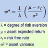
Risky asset weight (ω) formula
Rebalance
Describe, benefits, approaches (how/when), considerations
Describe: Rebalancing is adjusting systematically the portfolio when weights drift away from target due to price changes.
Benefits: Disciplined rebalancing means a more stable risk. Never rebalancing allows the high-return asset to dominate the portfolio, negating the benefit of diversification. It is a contrarian (countercyclical) strategy, were you sell winners to buy losers, sticking to the defined strategy.
Approaches: Calendar rebalancing (periodic basis); Percent-range rebalancing (define a % corridor - eg. 10% from 45% to 55%)
Considerations: Illiquid inv complicate reb.; Derivatives can synteticaly rebalance; taxes and transaction costs discourage reb; Risk-averse inv have tighter ranges.
MVO Objective function (Utility for asset mix)
Um = E(Rm) − 0.005 * λ * σ2m
Certainty-equivalent return (comparable to the risk-free**)
where
Um = utility for asset mix
Rm = return for asset mix
λ = the investor’s risk aversion coefficient - investor’s risk-return trade-off (how much inv will forgo return for lowering risk). 0 = risk neutralç 4 = risk moderate
σ2m = expected variance of return for asset mix m
eg.
6% = 10% - (0.5 * 2 * 4%) … atenção para o fator, que vira 50% se tudo estiver em termos %
SFRatio
SFRatio = [E(RP) - Rthreshold] / σP
Criticisms of MVO
- Output is highly sensitive to changes in inputs (especially returns)
- Highly concentrated asset class weights due to MVO preference for high Sharpe ratio assets (real estate before de-smoothing
- Fails to address other concerns such as skewness & kurtosis
- Source of risk may not be diversified (inflation, vol, etc)
- Fails to address liabilities or cash outflow
- Single period framework that does not account for trading and rebalancing costs
- Multi-period models are more comprehensive & complex
Addressing MVO criticism #3
Budget Constraints
(Problem solved, approach)
Budget Constraints
Problem solved: Improve input quality and add real-world constraints to the portfolio (eg. when you include non-tradable assets to the optimization and wishes to fix a % to them)
Approach: i. Set allocation; ii. range; iii. upper limit; iv. relative allocation to another asset class; v. liability-relative. CAUTION: imposing too much constraints is similar to stop optimizing the model.
Addressing MVO criticism #2
Black-Litterman
(Problem solved, approach)
Black-Litterman
Problem solved: Improvement over the reverse-optimization, creating a stable, MVO portfolio that overcomes expected return input sensitivity by providing a disciplined way to tilt inputs
Approach: Starts with the returns from the reverse opt (based on the mkt weights) combining with the analyst’s view (tilts) using absolute values for an asset class (eg. x expected return is 10%) or differentials to another class (eg. x will outperform y by 100bps)
Addressing MVO criticism #5
Non-Normal Optimization
(Problem solved, approach)
Non-Normal Optimization
Problem solved: Mean and variance are incomplete measures of risk. In a normal dist, there is no skewness (asymmetrical distribution) or kurtosis (frequency of extreme events), but asset class returns are not normally distributed and it may be the investor’s preference accounting for a non-normal distribution (prospect theory - investor’s pain of loss is 2x higher than joy from gain).
Approach: MVO using semi-variance, cVaR, mean-variance skewness, mean-variance-skewness-kurtosis
Addressing MVO criticism #4
Resampled MVO optimization
(Problem solved, approach)
Resampled MVO optimization
Problem solved: More diversified asset allocations
Approach: Combines Markowitz`s MVO with Monte Carlo to find the true population of the portfolio w/ a starting point in historical data and simulating scenarios (that account for skewness and kurtosis). Returns more diversified and stable ports, but can present concave bumps, over-diversification, susceptible to input errors and lacks theoretical support.
Addressing MVO criticism #1
Reverse Optimization
(Problem solved, approach)
Reverse Optimization
Problem solved: Input sensitivity of MVO - anchors expected return based on CAPM
Approach: Begins from the end. Uses optimal asset class weights (eg. mkt cap), covariance and risk aversion coefficient to solve for expected asset class return. With that E(r), find the portfolio that reaches this objective.
- *Risk Budgeting**
- “use risk efficiently in the* persuit of return”
Marginal Contribution to Risk (MCTR)
Absolute Contribution Total Risk (ACTR)
% Contribution to Total Risk
Ratio of Excess Return to MCTR
Marginal Contribution to Risk (MCTR) =
Asset Class β x Portfolio σ
Absolute Contribution Total Risk (ACTR) =
Asset portfolio weight x MCTR
total sum is equal to the portfolio’s risk
% Contribution to Total Risk =
ACTR / Portfolio σ
Ratio of Excess Return to MCTR =
(Asset exp. return - Rf) / MCTR
equal for every asset in the portfolio when allocation is optimal
Liability-Relative asset allocation
Surplus / Funding ratio
Surplus = MVAssets - PVLiabilities
Funding ratio = MVAssets / PVLiabilities
Surplus Objective function (Similar approach to MVO; Utility for asset mix)
ULRm = E(Rs,m) − 0.005 * λ * σ2m * (Rs,m)
Mix that maximizes expected surplus net of a penalty for surplus return volatility
where
ULRm = Surplus utility for asset mix
Rm = surplus return for asset mix
λ = the investor’s risk aversion coefficient - investor’s risk-return trade-off . 0 = risk neutral 4 = risk moderate
σ2m = expected variance of return for asset mix m
Two-portfolio approach
Approach, limitations and alternatives (+ agressive)
(conservative - used for DB and Insurance companies)
Part 1. Hedge liabilities - asset that match CF / duration / factors (eg. inflation) of liability
Part 2. Surplus invested at the return-seeking portfolio
Surplus required for the two-portfolio approach. True hedge may not be available (basis risk).
Partial Hedge and Dynamic Hedge are more aggressive approaches that do not fully hedge liabilities
Comparison b/w Liability-Relative Asset Allocation
Surplus Optimization vs Hedging/Return Seeking vs ALM (Integrated Asset-Liability Mgt)
ps1: Surplus optimization and two-portfolio approach, being single period models, have difficulty estimating probability of meeting future obligations
ps2: Surplus optimization considers the asset allocation problem in one step; the hedging / return-seeking portfolio approach divides asset allocation into two steps

Integrated Asset-Liability (ALM) Approach
(eg. insurance companies and banks)
Used when decisions regarding the liabilities composition is made in conjunction with the asset allocation.
More complex, multiple period liability model
For Insurance Companies - Liabilities difficult to hedge (eg. environ. risk); evaluate tail risk (eg. 1% VaR); form a diversified portfolio of liabilities
For Banks - Assets (loans) are jointly evaluated w/ liabilities (deposits); link asset perf w/ changing liability values
Goal-Based Asset Allocation
Objective, Approach (steps), What to do with the Surplus?
Individuals often have multiple goals.
Objective: Creation of sub-portfolio (modules) designed to address each goal individually over a specific time horizon and required probability of success (“urgency” level)
Approach:
1 - Define investor goal. Positive (wish to achieve, need, want, dream) or negative (seek to avoid, fear, worry, concern)
2 - Determine time horizon
3 - Required prob of success (dependent on keywords)
4 - Calculate the necessary funding for each set of goals based on the highest discount rate for a CF determined as the asset return for a specific time period and prob
5 - The aggregate portfolio will be the result of the weighted average of the % invested in each module by the respective exposure to different asset classes
Surplus: In the presence of a surplus after goal`s allocation, the investor would invest the money in a module for the interim period and may wish to (1) revaluate probabilities, (2) bring time-frame closer or (3) create new goal
Heuristic asset allocation
5 strategies that simplify allocation
120 minus your age (exposure to equity) - linear decrease
60/40 stock/bond - equity long term growth and bond diversify risk
Endowment Model - large allocation to non-traditonal assets (earn illiquidity premium and focus on active mgt) / contrast to Norway model
Risk Parity - each asset class contributes equality to risk (ignores the expected return) - distributes equally the risk b/w assets in a port
The 1/N rule - Equally weighted asset allocation (less exposed to input errors)
Asset Allocation Constraints - Asset Size
Economies & Diseconomies of scale
Large portfolios - size may constrain allocation to active/alpha equity strategies (increase in trade size, price impact, outside core thesis)
Large asset owner - Too small allocation may not meaningfully contribute to overall port return & risk
Small asset owners - Limited governance, Eligibility restrictions, Inadequate diversification, Inability to develop expertise
After-tax Portfolio Optimization
Return, Risk and Rebalancing Range
After-tax return
rat = rpt * (1 - t)
rat = pdividendrpt * (1 - td) + pcapital gainsrpt * (1 - tcg)
After-tax risk (std dev)
σat = σpt * (1 - t)
After-tax rebalancing range
Rat = Rpt / (1 - t)
Behavioral Biases in Asset Allocation
AA impact and Mitigators


